Statistical Hypothesis Testing and Confidence Intervals

By completing this section, you will be able to

Identity the two statistical hypotheses
Describe the relationship between scientific and statistical hypotheses
Identify the four possible outcomes of statistical decisions
Explain what $\alpha$-level and p-value have to do with statistical hypotheses
Conduct a one-sample z-test
Construct and interpret a 95% confidence interval

Professor Weaver’s Take

Life is full of decisions. We sometimes have the fortune of learning that we made a good decision. Other times we find out that we made a bad decision. Most of the time, we don’t get the luxury of knowing if we made the right decisions. Statisticians live in this realm of uncertainty. You will have to decide if the sample data you have say anything important about the population of interest. Luckily, there are some guidelines to help you made a decision but there is no such thing as 100% certainty in Statistics (maybe in life as well). In this section, how statisticians assess the risk of making incorrect decisions, the guidelines for an acceptable amount of risk and various ways of expressing our statistical inference.

Statistical Hypotheses

The goal of science is to generate knowledge. We hope to know how things happen, how things are related and how we can intervene in these processes. There are some important steps between generating questions and generating knowledge, some of which is the focus of this section. Before we get into the specifics of statistical hypotheses and decision making, let’s review the scientific method.

The Scientific Method

Following the scientific method for any one study does not guarantee knowledge. However, when we repeatedly use this methodical approach to try to understand the world, we can replicate and extend on previous results. Just as many or larger samples better approximate the population, we hope that many studies can help us see the underlying truth of some phenomenon. Figure 10.1 highlights the cyclical steps of the scientific method.

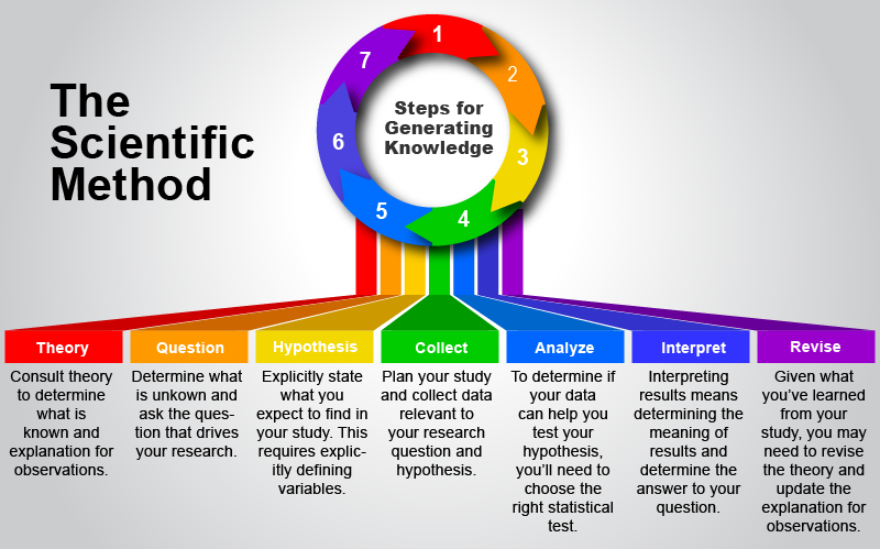
Figure 10.1. Cyclical steps of the scientific method

Steps of the scientific method:

Consult Theory

Very often, there is an existing account of observations and their relationships. When possible, you should consult existing theory to guide you to the important questions that need investigation.

Form Research Question

The research question is the guiding focus of the study. It may often be stated in general terms before operational definitions (how concepts will be measured) are developed.

Derive Hypothesis

With the question in place and with the background information from theory, you can state your best guess about the outcome of the study.

Collect Data

The planning is done and now it’s time to collect the data relevant to your question and to test the hypotheses.

Analyze Data

As you’ll learn in the remainder of this course, your selected analyses will be dependent on the type of data collected, the research question, and the assumptions of the analytical procedures.

Interpret Results

Can you answer the research question? Did you find support for your hypothesis? This is the focus of the current section.

Revise Theory

If you’ve found something that can help answer a question derived from the current theory or perhaps your work introduces new questions, you will need to integrate the new information with the existing theory.

The scientific hypothesis is one’s expectation about a specific outcome. For example, one might hypothesize that, given the mass of the moon, an object would fall at a rate of 1.67 m/s². The two statistical hypotheses are much more general and are completely inclusive.

Two Statistical Hypotheses

In statistical inference, we have two hypotheses. The null hypothesis (represented as H₀) states that there is no difference between groups, no relationship between variables, no difference between populations, or whatever statistical effect you are investigating.

The Null Hypothesis (H₀) states that there is no effect.

This is the default assumption for statistical analyses. It is not because we are pessimists but because we want to have enough evidence for a claim rather than assume some effect. It is like default assumption in the U.S. justice system: innocent until proven guilty. This tradition has its roots in the wiring of Renee Descartes who argued that one should never assume anything and should prove everything.

There is a complementary hypothesis, the alternative hypothesis (represented as H_a), which states that there is an effect, relationship, etc. That is quite the general statement.

The alternative hypothesis (H_a) states that there is an effect.

This hypothesis is not the same as the scientific hypothesis because it only predicts that there is something happening but does not predict a particular value. Most specifically, we can form a directional alternative hypothesis. This version of the alternative hypothesis states that we may expect a positive versus a negative relationship, or perhaps that our sample represents a population that has a mean greater (versus lesser) than some other value. Although it is generally better to be more specific, I suggest that you stick with the more general version of the alternative hypothesis. I will provide more information on this shortly, but for now just remember that the more inclusive version ensures that you won’t miss something important by restricting your prediction to just one direction.

Decisions and Errors

Given that we start off assuming that our analyses will match the H_0_ (the null hypothesis), we have two possible decisions following our analyses. We can choose to overturn or reject the H₀ or we can choose to keep or retain the H₀ (note that this is not “accepting the null hypothesis”). Essentially, if we find that our data does not match the H₀ very well, we should reject that in favor of the H_a (we’ll cover how you might make this decision in the next bit). Of course, our decision may be in error. Table 10.1 highlights the decisions and outcomes of those decisions.

Table 10.1

Confusion Matrix for Statistical Hypotheses

		State of the World
		H₀ True	H₀ False
Decision	Retain H₀	Correct Decision (1-$\alpha$)	Type II Error ($\beta$)
	Reject H₀	Type I Error ($\alpha$)	Correct Decision (1-$\beta$)

Our two correct decisions occur when our decision matches the state of the world (what is really happening in the population). We can also make one of two errors. The Type I error (represented as $\alpha$) occurs when we think that we’ve found some effect but there is no effect. We can also refer to Type I errors as False Positive Errors because we are incorrectly concluding (false) that we have a finding (positive). A Type II error (represented as $\beta$ occurs when we do not think that there is an effect when there is an effect in the population. Type II errors are also called False Negative Errors. As you may imagine, we try to minimize the errors and maximize the correct decisions. This can be a little tricky given that we are only able to estimate what is happening in the population base on what we observe in our samples. As such, we will look at the probability of making an error or making a correct decision. Statisticians like to minimize Type I errors ($\alpha$) and to maximize when we correctly reject the H₀ (1-$\beta$). Before we discuss how to do this, we should translate these terms back into a familiar framework of the normal distribution and probability.

Decisions, Errors, Distributions and Probability

To make this a little easier, let’s give ourselves some context with the following example. We are pricing airline tickets for a Spring Break trip so we are looking through various websites that claim to offer the best price for tickets. You heard on the news that the average airline ticket price in the U.S. is $371.00. You wonder if these websites are any different than the national average. We now have some information to get us started.

The null hypothesis is that there is no difference between our sample’s estimate for the population and the population parameter. As such, we assume that our sample average from the websites will be equal to the national average. Stated in short form:

\[ H_0 : M = \mu_0 = \$371.00 \]

We can make a sampling distribution that has M = $\mu_0$ at the center (figure 10.2)

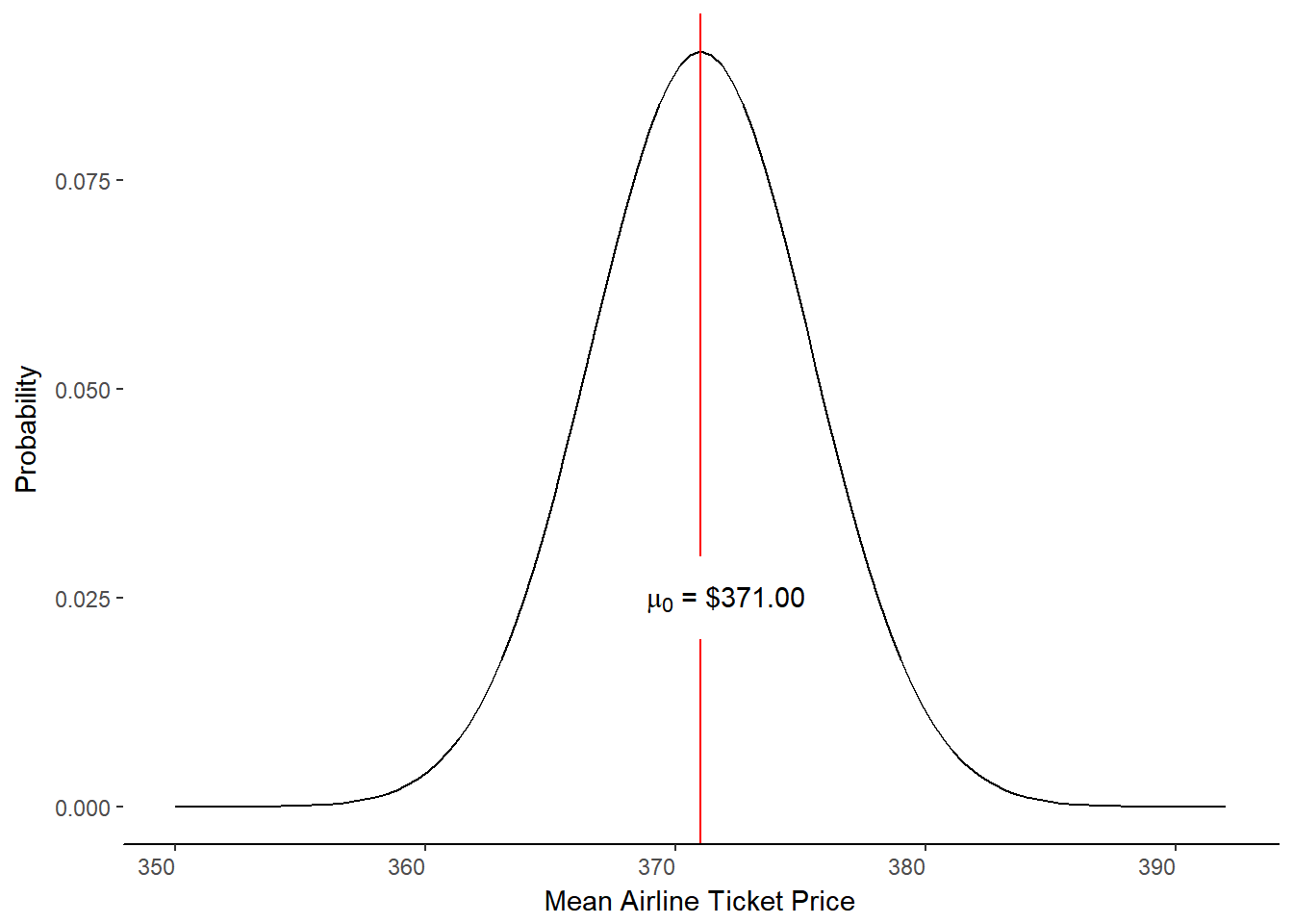
Figure 10.2. The Null Hypothesis Distribution.

Given we have a normal sampling distribution, we can easily determine the probability of getting other sample means than the hypothesized population mean. For example, if we assume that our population standard deviation is $\sigma$ = $44.13 and a sample size of 100, we could easily determine z-scores for different sample prices.

Let’s find out the how much the 10% most expensive samples would be. We need to work this problem in reverse. That means we have to find the z-value associated with a probability of p = 0.10 beyond the z-score (i.e., in the tail). We can find that information in column C or the (unit normal table)[http://webp.svsu.edu/~jweaver/Tables/UnitNormalDistribution.html]. The z-value where 0.10 of the area under the curve is to the right is 1.2816. Next, we need to convert this z-score into the average ticket price for that sample by plugging our known values into the z-score formula.

\[ \begin{aligned} z &= \frac{M-\mu}{\frac{\sigma}{\sqrt{n}}} \\ 1.2816 &= \frac{M-\$371.00}{\frac{\$44.13}{\sqrt{100}}} \\ 1.2816 &= \frac{M-\$371.00}{\$4.41} \\ 1.2816 \times \$4.41 &= M-\$371.00 \\ \$5.66 &= M-\$371.00 \\ M &= \$5.66+\$371.00 \\ M &= \$376.66 \end{aligned} \]

A travel site that yields an average ticket price of $376.66 would be more expensive than 90% of all sites. Would that be expensive enough for us to think that this site is selling tickets with a different set of prices or could we just consider it a natural fluctuation in ticket sales? We need some type of decision rule.

In the social sciences, we believe that any sample that is 1.96 standard deviations above or below the null hypothesized value ($\mu_0$) is unlikely to be part of the null hypothesized distribution. That is, it reasonable to assume that the sample was drawn from some other population of values. Thus, we should reject the H₀

A z-score of greater than 1.96 or less than -1.96 is considered to be too extreme, leading to a rejection of H₀

Why a z-score of 1.96? This corresponds to the most extreme 5% of the null hypothesis distribution. When we divide the 5% across the two tails of the distribution, we call it a two-tailed test. It is extreme/unlikely enough that we might believe the sample came from another population but the chances of making a Type I error ($\alpha$) are low enough to be acceptable. To minimize $\alpha$, we only reject the null hypothesis if there is less than a 5% chance of making a false positive claim. If the null hypothesis is correct, that leaves a 95% chance of correctly maintaining, or failing to reject, the null hypothesis (1-$\alpha$).

We only reject H₀ if there is less than a 5% chance of getting that value (or more extreme) for the null hypothesis distribution. We typically use a two-tailed test of the null hypothesis by checking for extreme values in each tail of the distribution.

We can now make our decision to reject or retain the null hypothesis by either converting to z-scores or by determining the area under the curve beyond mean (column c). All things considered, you’ll save yourself a step by just remembering that Z=1.96 corresponds to an $\alpha$-level of 0.05. Stated differently, the probability of obtaining a mean with a z-score of 1.96 or greater is 0.05.

To summarize, if a the z-score from our sample is greater than 1.96 or less than -1.96, we reject the null hypothesis. However, if our obtained z-score is between -1.96 and 1.96 (including those values), we fail to reject the null hypothesis. Figure 10.3 adds these criteria to the null hypothesis distribution and adds the decisions to the various areas of the distribution.

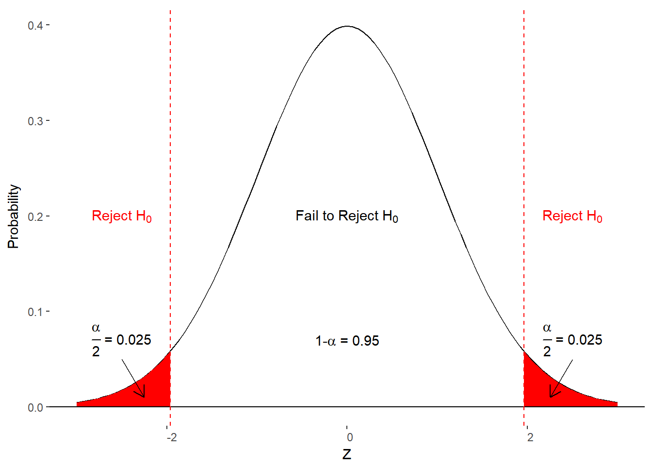
Figure 10.3 Criteria, decisions, and outcomes under the null hypothesis.

We will follow these basic rules for all of statistical hypothesis testing for this course.

Wait. All of this was about the null hypothesis and the resulting distributions of sample means. What if the alternative hypothesis is the truth? That is, what about Type II error ($\beta$) or a false negative error. This would occur if our sample was really from a different population than the null hypothesis distribution but we fail to detect it. Figure 10.4 illustrates where this can occur.

Figure 10.4. A Type II error with the null and alternative hypotheses distributions.

If $\beta$ is the probability of making a Type II error then 1-$\beta$ is the probability of correctly rejecting the null hypothesis. Another term for this is statistical power. It is the power to detect an effect, difference, or relationship if it exists. As you might imagine, statisticians like to maximize statistical power.

Factors impacting statistical power.

According to figure 10.4, statistical power is the area under the alternative hypothesis curve to the right of our boundary for $\alpha$. To increase the proportion of the area under the curve that we consider statistical power, we have a few options.

Increase $\alpha$ (moves boundary to left)

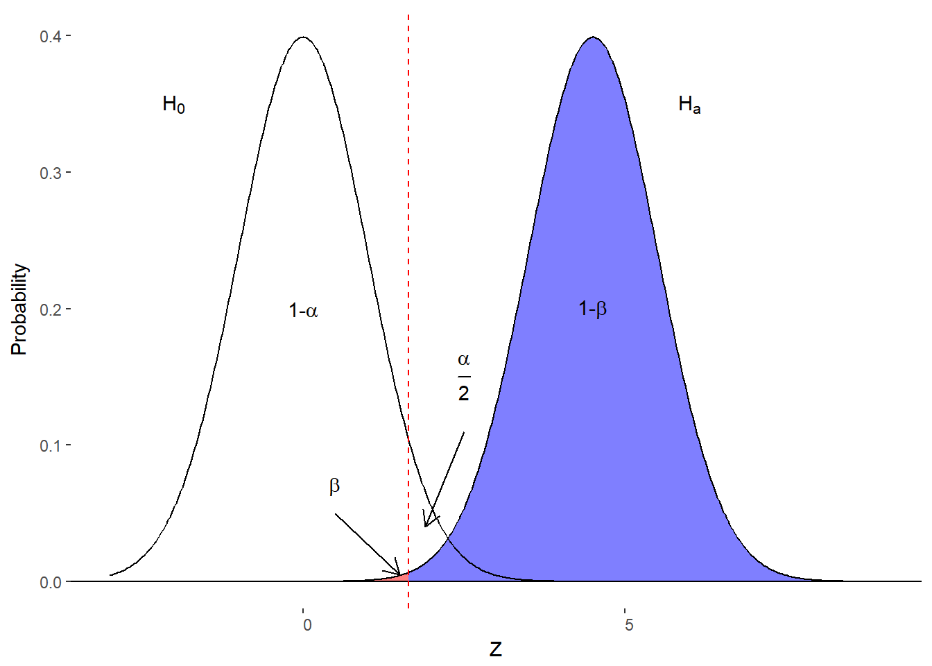
Figure 10.5. Effect of increasing $\alpha$

Increase space between Distributions

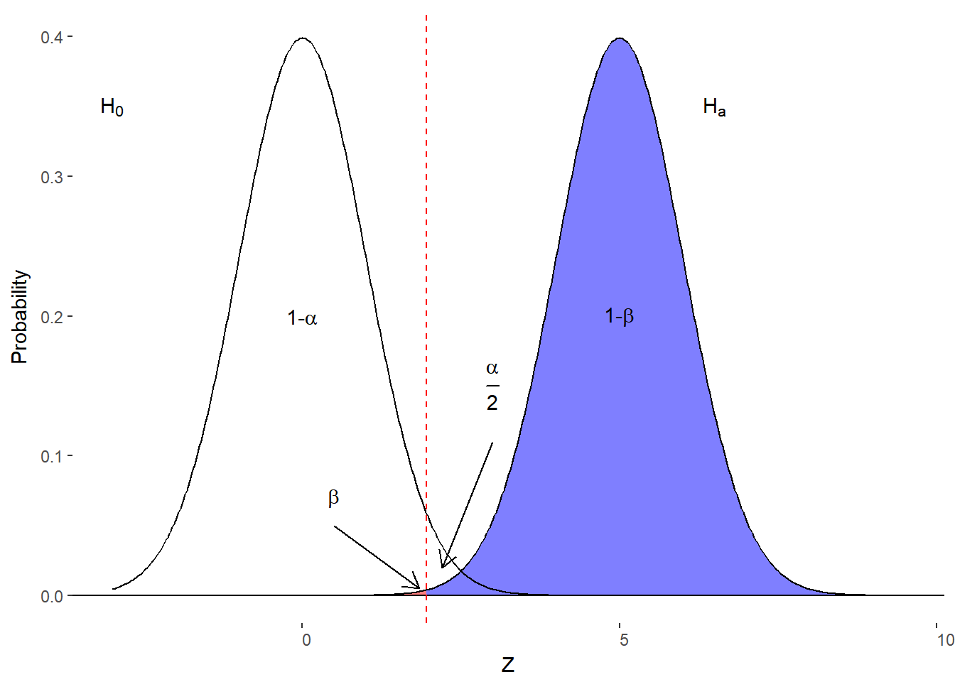
Figure 10.6. Effect of increasing effect size

Decrease variability of distributions

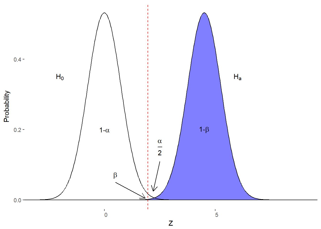
Figure 10.7. Effect of decreasing variability

Although all of these optics have the desired outcome, only one is a practical solution. We cannot increase our Type I error rate and we cannot change the reality of the population values (i.e., mean of sampling distribution). We can however reduce variability of those distributions. Recall that the variability of a sampling distribution of sample means is the standard error of the mean. The standard error of the mean is equal to the population standard deviation divided by the square root of the sample size.

\[ \sigma_M = \frac{\sigma}{\sqrt{n}} \]

We cannot affect the population variability, but we can increase our sample size. The larger the sample size, the smaller the standard error of the mean, the tighter the distributions.

I had made a note to you earlier that failing to reject or maintaining the null hypothesis is not the same as accepting the null hypothesis. The reason is we often don’t have enough evidence to suggest that our sample mean is statistically equivalent to the hypothesized population mean. That is, there is a high probability of making a Type II Error ($\beta$). As we are now discussing, we attempt to maximize statistical power so that we have a good chance of detecting an effect if it exists. So, if we can maximize power (1-$\beta$), we are minimizing $\beta$ and thus giving us more evidence that the null hypothesis may be true if we don’t reject it. In general, the social sciences aim for power = 0.80 or better. Studies often fail to achieve this for various reasons but it is important for making sound statistical conclusions because a low powered study may be reporting spurious results.

Now that we know about our available decisions, potential errors and how we control or maximize our outcomes, it is time to put it into practice.

Hypothesis Testing: One-Sample Z-test

The goal of null hypothesis significance testing (NHST) is to make a decision regarding the null hypothesis. That is, we need to determine if the data we obtain suggests that the null hypothesis should be maintained or rejected. We do this by comparing our obtained value to some critical value (e.g., z-score) or by comparing the probability of obtaining that value (i.e., the p-value from column C) to our $\alpha$-value. Let’s build up our airline ticket example with all of the necessary information.

As you may recall, we are curious about the representativeness of travel site airline ticket prices. Our research question could be “do travel sites charge the typical amount for airline tickets?” Notice how this is phrased; we are not suggesting that the sites charge more or less - just different. This is a two-tailed alternative hypothesis.

The Bureau of Transportation Statistics ¹ reports that the national average ticket price in the U.S. $ 437.19 in the fourth quarter of 2017. Because we assume H₀ to be the truth in the world, our null hypothesized value for our population of tickets taken from the travel sites is $\mu_0$= $ 347.33 The dataset from the BTS also reports a standard deviation for the ticket prices ($\sigma$ = $ 158.57).

Unfortunately, we don’t have the time to check every travel site so we just pick the top result from a search engine and use the ticket information from that site. We sample 1,0000 tickets from the website and get an average ticket price of (M=) $ 503.27. We can easily see that this price is higher than the national average ($ 503.27 > $ 347.33) but we also know that there is some variability in those national prices ($\sigma$ = $ 158.57). Is the website price extreme enough for us to consider it to be from another distribution of ticket prices? We will have to compare some values.

Method 1: Compare obtained z-score to critical z-score

Recall that our critical z-score for a two-tailed test is z = 1.96. That is, any obtained score more extreme than 1.96 (or -1.96) has a less than 5% ($\alpha$) chance of being from the null hypothesis distribution. We’ll need to convert our travel site mean ticket price into a z-score to do this comparison.

\[ \begin{aligned} z &= \frac{M-\mu_0}{\frac{\sigma}{\sqrt{n}}}\\ z &= \frac{503.27 - 347.33}{\frac{158.57}{\sqrt{1000}}}\\ z &= \frac{155.94}{5.01}\\ z &= 31.13 \end{aligned} \]

Our obtained z-score (z_obt) is 31.13. Let’s plot our critical value and obtained value on the null hypothesis distribution (figure 10.8). Because z_obt lies outside of our critical z-scores (z_crit), it is in the reject H₀ zone.

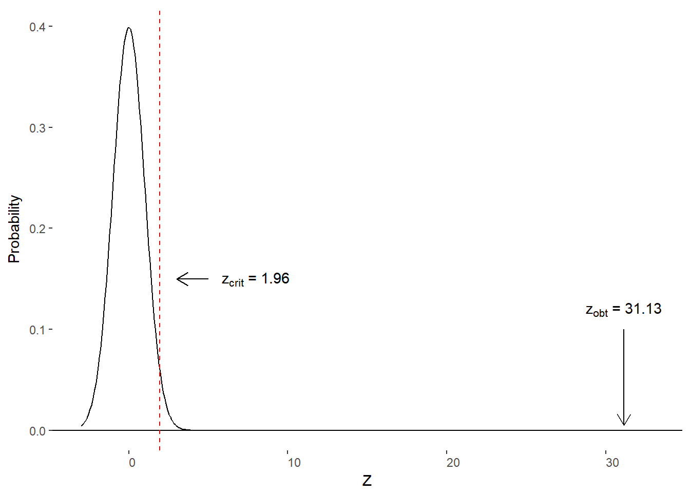
Figure 10.8. Critical and obtained z-scores

Method 2: Compare p-value to $\alpha$-level

Just as with method 1, we will need our sample mean converted to a z-score.

\[ z_{obt} = 31.13 \]

We will then need to find the area under the curve to the right (column C). Unfortunately, our table stops at 4.00. We can either use a statistical program to give us an exact value, or we can state that p(z=31.13) > .0001 as p(z=4.00) = 0.0001. We can compare the obtained p-value to our $\alpha$-value. Given that our p-value is less than our $\alpha$-value (0.0001 < 0.05), we reject H₀.

State conclusion

We’ve made the same decision using either method (comparing z-values or comparing p to $\alpha$). The next step is to formally state our conclusion. To be clear, the decision regarding the null hypothesis is not the same as the conclusion. The conclusion is the answer to our research question. When we reject H₀, we can give an answer to the research question. In our example, we can conclude that the travel site sells tickets at a higher price than the national average.

The conclusion is the answer to the research question informed by the results of statistical analyses.

What if we fail to reject H₀? If you have high statistical power, you could claim that the null hypothesis is true. For example, you may report that the travel sites sell airline tickets at national average prices. However, if you do not have sufficient statistical power, you have to conclude that the results are insufficient. You would write that “failing to reject the null hypothesis and the lack of statistical power yields ambiguous results. Travel sites may be charging ticket prices other than the national average but this study did not detect this.”

It is always important to state your conclusion with the limitations in mind. Overstating your conclusions is bad science. There is room for discussion about possible implication of results, but you should not speak in absolutes. After all, statistical inference is done through estimation and assessing probability of error.

Confidence Intervals

Null Hypothesis Significance Testing (NHST) can tell us if our result is unlikely due to chance variation in our sampling. That is, it can tell us that our sample is unlikely to have come from our hypothesized population. This is useful and has dominated most of social science statistical analyses for many decades. This approach is limited. What if we wanted to know what values we could expect from the population from which our sample was derived. Rather than just the basic “yes” or “no” response from NHST, confidence intervals can tell us the potential sample values that we would obtain on repeated sampling from the population. We’ll find that we can also use this information to do NHST.

Confidence intervals are the expected values to be obtained from repeated sampling with samples of the same size.

Confidence intervals are associated with a particular level of confidence and that level of confidence is 1-$\alpha$. Although it is customary to stick with the alpha established for a particular field (e.g., 1-$\alpha$ = 1-.05 = .95), you can vary the level of confidence. There is a bit of a trade-off for increasing the confidence for the interval. The higher the confidence, the wider the range (less precision). However, if you want a more narrow range (more precision), you’ll have less confidence. That is, you can be 100% certain that your samples will have a mean betwen $-\infty$ and $+\infty$ or you could pick a small range, say between $ 502.00 and $ 503.00 but only have 1% confidence. We’ll stick with they typical $\alpha$ of 0.05 and construct a 95% confidence interval. This will allow us to nicely tie back into NHST.

Calculate Confidence Interval

The good news is that we don’t need any extra information than we used for NHST. We’ll need the following information for a confidence interval

Sample Mean
Critical z-score
Standard error of the mean

From those numbers we’ll derive the upper and lower bounds of the interval using the following formulas

\[ \begin{aligned} CI_{lower} = M - z_{crit} * \sigma_M \\ CI_{upper} = M + z_{crit} * \sigma_M \end{aligned} \]

This shows that we are centering our confidence interval on the sample mean, which is our unbiased estimator of the population mean. We then add on what is known as the margin of error ($z_{crit}*\sigma_M$). The margin of error is the amount of change in the estimate expected for the confidence interval. It is the same as you’ll find in a presidential election poll. For example, if you read that Smith leads Johnson by 10 points with a 3 point margin of error, you can expect the lead to vary between 7 and 13 points with other samples of the same size.

Let’s calculate the 95% CI for our airline ticket example. From our work earlier, we have the following values.

M = $ 503.27
z_crit = 1.96
$\sigma_M$ = 5.01

If we plug that information into our equations, we get:

\[ \begin{aligned} CI_{lower} & = M - z_{crit} * \sigma_M \\ &= 503.27 - 1.96*5.01\\ &= 493.45\\ CI_{upper} &= M + z_{crit} * \sigma_M \\ &= 503.27 + 1.96*5.01\\ &= 513.09\\ \end{aligned} \]

We write the results as 95% CI [493.45, 513.09]. We interpret the results as 95% of all samples of tickets of n=1000 would yield a mean airline ticket price between $ 493.45 and $ 513.09.

Confidence Intervals and NHST

Now that we have our confidence interval bounds, we can test if our samples are inline with the expected population mean. This is essentially the same process as before except we are switching perspectives. Rather than focusing on the null hypothesis distribution on which we place our sample mean, we will put the null hypothesized population mean ($\mu_0$) onto the alternative distribution. If $\mu_0$ is outside of the bounds of the confidence interval, we will reject H₀. If $\mu_0$ is inside of the bounds, we will maintain / fail to reject H₀. Figure 10.9 compares the two approaches.

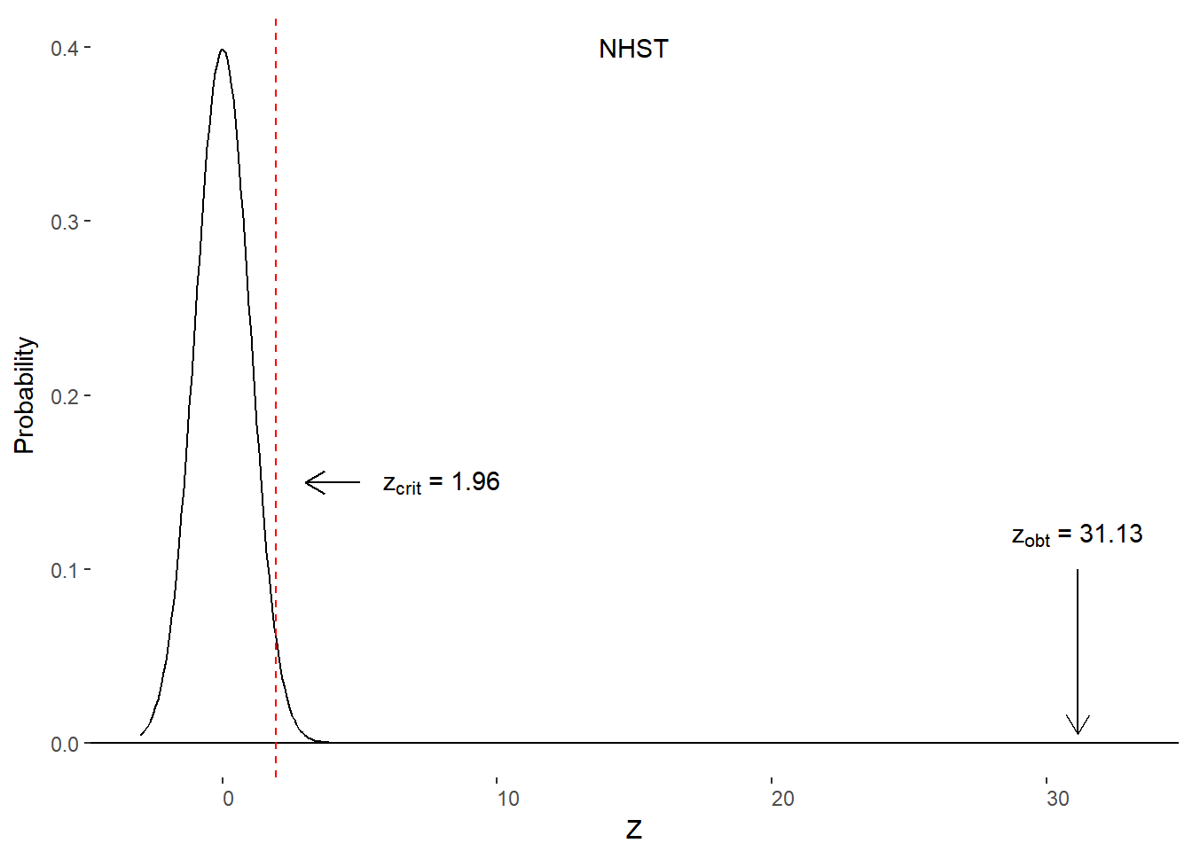
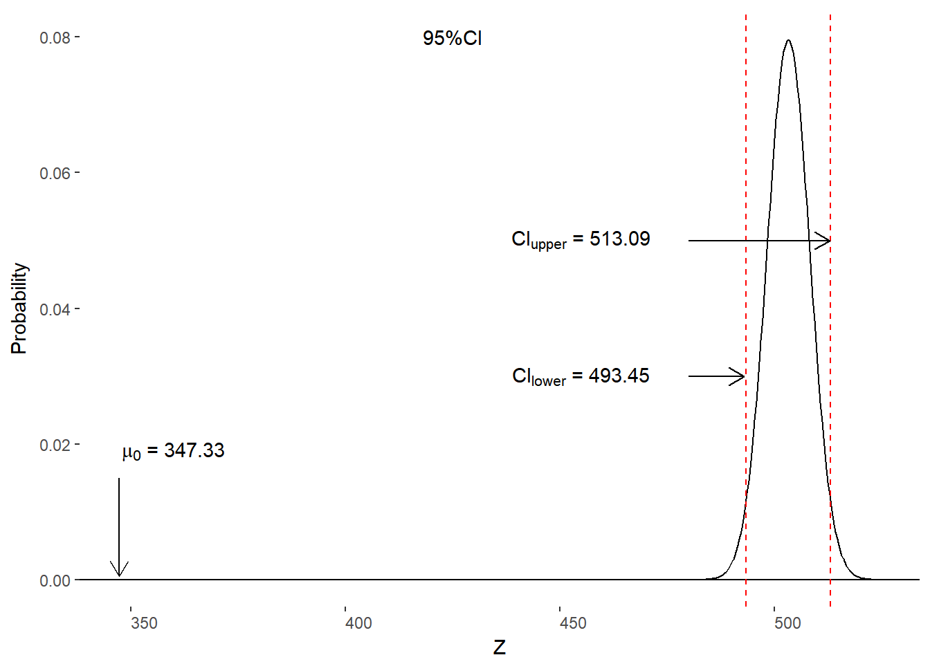
Figure 10.9. Comparison of NHST and confidence interval approaches to testing H₀.

Recall that $\mu_0$ = $ 347.33 and that our 95% is [493.45, 513.09], which means that our $\mu_0$ is outside of the 95% CI and we should reject H₀. This is the same decision we reached using NHST in earlier parts of this chapter.

Summary of Confidence Intervals

Confidence intervals provide the upper and lower bounds of the range of possible sample means (of the same size).
The confidence (e.g., 95%) relates to the expected portion of samples to yield values within the confidence interval.
You can perform NHST by comparing $\mu_0$ to the CI.
- If $\mu_0$ is inside of the CI, fail to reject H₀
- If $\mu_0$ is outside of the CI, reject H₀.

Where we are going

It has been a bit of a journey to get to this very important place. We have discussed various types of data and scales of measurement in an effort to describe data from a sample. We also discussed the various ways in which we might summarize that information. Now, we are taking that information about a sample in an attempt to generalize to a population. The first step was to construct a sampling distribution. The second step, and the focus of this section, was to make a judgment of the likelihood of some sample mean for a distribution of sample means from a hypothesized population.

The rest of the course will apply all of this information to special cases. Up next, the t-test, which is used when we want to judge if one or two samples came from different populations but we have to estimate the population variance. Following that, we’ll explore the Analysis of Variance (ANOVA) to determine if more than two groups came from different populations. We’ll end the course by determining if two variables are related in a population through correlation and regression analysis. Although this may sound ambitious for the rest of our time, it will be an easy task if we have mastered these basics.

References

United States Department of Transportation. (2018). Average domestic airline itinerary fares by origin city for Q4 2017 ranked by total number of domestic passengers in Q4 2017 [data file]. Retrieved from: https://www.transtats.bts.gov/AverageFare/↩