By participating in this section you will be able to:
- Explain the need for the family of t-tests.
- Describe the parameters of the t-distribution.
- Compute a t-value
- identify the key difference between the one-sample z-test and the one sample t-test
- Differentiate between the one-sample, between-subjects and within-subjects/matched-paired t-tests
- state the assumptions of each test
- Perform null hypothesis significance testing
- Calculate 95% confidence intervals
Professor Weaver’s Take
We’ve come really far in this course. We started with a basic description of statistics and now we’re amassing the techniques that will allow us to make some informed decisions about data and give answers to research questions about that data. The last chapter gave us a good foundation for asking and answering statistical questions but we’ll soon find that our vision of the world was too simplistic. As we move through the rest of the course, we will need to learn ways to adjust or approaches for different situations that require new assumptions or correct for faulty assumptions of earlier tests. Such is the case for the t-test.
What Is Wrong with Z?
We all like Z-scores. I wish everything worked with a one some z-test because we’ve got the formula down and we know how to use the table. Unfortunately, the z-test is only applicable in a very restricted case. That is, to use a z-test we must have the population standard deviation because we use that to calculate the standard error of the mean.
\[ \begin{aligned} Z &= \frac{M-\mu}{\sigma_M} \\ \sigma_M &= \frac{\sigma}{\sqrt{n}} \end{aligned} \]
It is rare that we have the population standard deviation but even if we did, we are only able to answer the following question: is the sample mean unlikely to be from the hypothesized population. Started anything way, we’re only able to ask about the representativeness of one mean for a population. This is a while question because it also allows us to create confidence intervals to make predictions about the true population mean from which the same was drawn.
There are other interesting and worthwhile questions that go beyond the z-test, however.
- Are the means from two samples from the same population (i.e., are two groups different)?
- Are the scores after some treatment different from before the treatment?
- Are multiple groups different on some measure?
- Are there scores from two variables related?
- What score on a dependent variable should we expect for someone with a given independent variable score?
We will cover the techniques used to answer the first two questions in this section with the rest to follow in subsequent sections.
What does T offer?
Variance Estimation Error
When we don’t know the population standard deviation (\(\sigma\)), we need to estimate it. Recall from sampling distributions that the mean of sample variances is the best unbiased estimator of the population variance. Unfortunately, we don’t have many samples from which to estimate the population variance. However, because the estimate is unbiased (sometimes under and sometimes over), any sample variance we use has an equal likelihood of being greater than or less than the population variance. That means our best guess available is our sample variance. There is a caveat, however, that also came with the sampling distribution of sample variances: the smaller the sample size, the worse the estimate. When samples are small (n < 1,000), we may be underestimating the population standard deviation. This bias leads to increased Type I errors because it results in a larger z-score than would occur if we had a larger population value. For example, imagine that he true population variance \(\sigma\) was 3 but a small sample size yielded an estimate of 2.
\[ \begin{aligned} \text{Estimate } & \text{vs. Actual} \\ \frac{3-9}{2} &> \frac{3-9}{3} \\ \frac{6}{2} &> \frac{6}{3} \\ 3 &> 2 \end{aligned} \]
Because of the larger z-score for the estimated variance, we would be more likely to reject the null hypothesis than if we had the actual population variance. The t-test was introduced to correct for the bias introduced when we erroneously assume we know the population standard deviation.
Family of T-distributions
To account for the problem underestimating population variance when using small sample sizes, the t-distribution varies in shape according to the degrees of freedom for the sample data.
Degrees of Freedom
Degrees of Freedom refer to the number of sample observations that can remain unknowable until observed. That is, because of the properties of the distribution and certain sample statistics, we will know at least one value in the sample if we observe all of the others. Let’s imagine that we have a sample with 5 values and a sample mean of 10. If we get the first 4 values, we will know the last value because we already know the mean
\[ \begin{aligned} M &= \frac{\Sigma x}{n} \\ 10 &= \frac{5 + 7 + 13 + 15 + x}{5} \\ 50 &= 5 + 7 + 13 + 15 + x \\ 50 &= 40 + x \\ x &= 10 \end{aligned} \]
In any case in which we are using a sample mean to estimate a population mean, we must subtract 1 degree of freedom from our total sample size. This reduced sample size is used to determine the shape of the t-distribution.
Degrees of Freedom are the values of a sample that are not fixed. They are equal to the sample size minus the number of estimated population means.
Remember that the smaller the sample size, the more error in our estimation of sample variance. If we have more potential error in estimating variance or standard deviation in the population, we should require stronger evidence to reject the null hypothesis. That is, the smaller the degrees of freedom, the larger the critical value needed to reject H0.
Figure 11. 1 shows a few t-distributions with the degrees of freedom (df) equal to 1, 5, and 1,000. Notice how the critical t-value associated with the top 5% of the distribution changes in relation to the the degrees of freedom. Also, as the sample size gets large enough (n ~= 1,000), the t-distribution becomes the standard normal distribution.
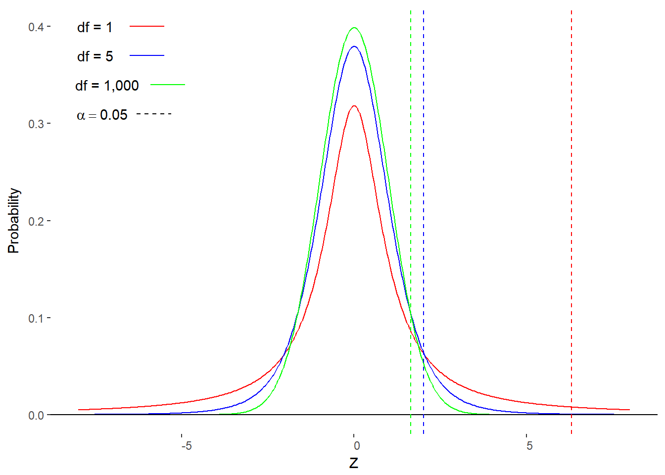
Figure 11.1. Three t-distributions (df = 1, 5, 1000) and associated critical t-values for \(\alpha\) = 0.05 (one-tailed).
The T-table
Finding the appropriate critical t-value is very easy when consulting the T-table. Figure 11.2 is an excerpt of the table to highlight the layout of the table.
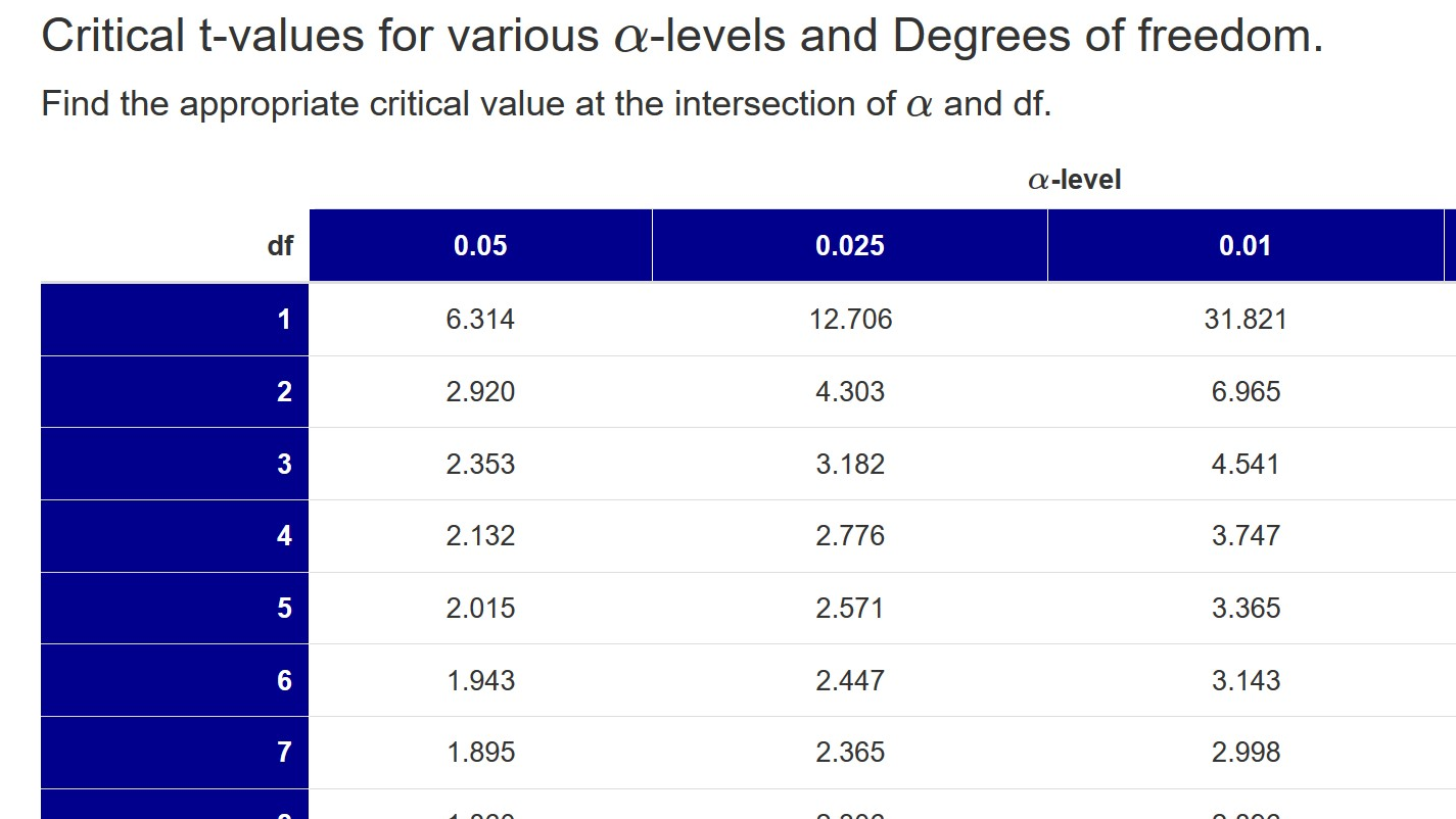
Figure 11.2. Excerpt of the T-table.
The top row of the t-table contains the alpha-level (\(\alpha\)) and the first column contains the degrees of freedom (df). The critical t-values are located in the cells at the intersection of a particular \(\alpha\) and df. Notice how the values in the table change. As maintain df but decrease \(\alpha\), the values increase. However, as you maintain \(\alpha\) but increase df, the values decrease. Check out the full table and find the critical t-value for df = 15 and \(\alpha\) = 0.025 (this is equivalent to a two-tailed test with \(\alpha\) = 0.05).
Steps for Finding the Critical T-value
- Determine the appropriate \(\alpha\) level.
If performing a two-tailed test, divide by \(\alpha\) by 2.
- Determine the degrees of freedom.
Subtract the number of sample means from the number of observations (n)
- Find the critical value at the intersection of df and \(\alpha\).
You may need to estimate the critical value or use statistical software if appropriate df and \(\alpha\) are not in table.
Now that we can account for sample size more appropriately and have a handy table with necessary critical values, let’s learn about the one-sample t-test.
One-Sample T-test
The one-sample t-test is analogous to the z-test. That is, we want to know if a sample mean is representative of some hypothesized population. The equations for the two are very similar with main difference between the two being how we calculate the standard error of the mean. Whereas in the z-test we assumed we had to know the population standard deviation, the z-test utilizes the sample standard deviation. The real impact lies within the table of critical values. For small sample sizes, the critical t-value will be larger than the critical z-value.
\[ z = \frac{M-\mu_0}{\frac{\sigma}{\sqrt{n}}} \] \[ t = \frac{M-\mu_0}{\frac{s}{\sqrt{n}}} \]
The steps of the two tests are equivalent.
Steps for the One-Sample T-test
- Determine the \(\alpha\)-level.
Are you performing a two-tailed test (please do!)? If so, divide \(\alpha\) by 2.
- Determine the df.
For one-sample t-test, df = n-1.
- Look up critical t-value.
Find at intersection of \(\alpha\) and df.
- Calculate t-value.
Use t-transformation formula.
- Compare calculated and critical t-values.
If calculated absolute value of t-value is greater than critical t-value, reject H0
- State conclusion.
Answer the research question given your decision regarding H0
Assumptions of the t-test
Although we are doing away with the assumption that we will always know the population standard deviation, there are a few important assumptions about the data we need to discuss.
Normality of population. The population from which each sample is derived is assumed to be normally distributed. We can check this assumption formally with statistical software but for hand calculations, you can give a rough examination of the histogram or bar chart. You can also compare the three measures of central tendency.
Random sampling. When collecting the sample from the population, it is assumed that those observations are random. This helps to collect a sample that is representative of the population.
Independence of observations. Each observation should be independent of any other observation. That is, the value of any observation should not impact any other observation. Random sampling can help to ensure this assumption is valid.
Example
You’ve recorded the height of (n=) 20 randomly selected female friends to find an average of (M=) 5 feet 6 inches or 66 inches and a standard deviation of (s=) 2.5 inches. The heights are roughly normally distributed. You’ve read that the average female height in the U.S. is 63 inches. Are your friends typical of the U.S. population?
Assumption Check
- Normality. We’ll assume this is the case, given the problem information.
- Random sampling. The problem information suggests that this is the case.
- Independence of observations. It seems hard to imagine that the height of one person can influence the height of another so we will maintain this assumptions.
Step 1. Determine the \(\alpha\)-level.
If we are not told, or have reason to, select a specific \(\alpha\)-level, we should go with our typical \(\alpha\) = 0.05. Should we perform a one-tailed or two-tailed test? The question asked if the friends are typical. It did not ask if they were shorter or taller. Therefore we should perform a two-tailed test. Actually, even if the question did ask if the friends were taller than suggested by the population, we should still perform the two-tailed test to test for the possibility that the friends are shorter. Better safe than sorry.
As such, our \(\alpha\)-level is 0.05/2 = 0.025
Step 2. Determine df.
Recall that the degrees of freedom are equal to the sample size minus the number of estimated population means. In this case, we are only testing one mean so we should subtract 1 from our sample size.
df = n - 1 = 20 - 1 = 19
Step 3. Look up the critical value.
With \(\alpha\) = 0.025 and df = 19, the table gives us a value of 2.09
Step 4. Calculate t-value.
Using the information provided and the t-transformation equation, we get
\[ \begin{aligned} z & = \frac{M-\mu_0}{\frac{s}{\sqrt{n}}} \\ z & = \frac{66-63}{\frac{2.5}{\sqrt{20}}} \\ z & = \frac{3}{\frac{2.5}{4.47}} \\ z & = \frac{3}{0.56} \\ z &= 5.36 \end{aligned} \]
Step 5. Compare values
\[ \begin{aligned} z_{calc} =& 5.36 \\ z_{crit} =& 2.09 \\ \\ z_{calc} >& z_{crit} \end{aligned} \]
Because our calculated z-value is greater than our critical value, the probability of making a Type I error is less than our \(\alpha\)-level. Therefore, we can reject the null hypothesis.
** Step 6**. State Conclusion
The rejection of H0 leads usto conclude that the heights of our friends are not typical of the U.S. female population.
Confidence Interval
Although null hypothesis significance testing (NHST) is still popular, it is recommended that you also provide a confidence interval for the range of likely population values. The process for creating a confidence interval is identical when using the t-distribution as it was for the z-distribution. The only difference is that you are replacing the critical z-value with a critical t-value.
Here is the updated formulas for finding the upper and lower bounds for a confidence interval: \[ \begin{aligned} CI_{upper} & = M + t_{crit}*\sigma_M \\ CI_{lower} & = M - t_{crit}*\sigma_M \end{aligned} \] We can confirm our NHST result with a 95% CI by checking if the null hypothesized mean (\(\mu_0\)) is included in the interval. Using the formulas for the limitis and the values calculated earlier, we find: \[ \begin{aligned} CI_{upper} & = M + t_{crit}*\sigma_M = 66 + 2.09*0.56 = 67.17\\ CI_{lower} & = M - t_{crit}*\sigma_M = 66 - 2.09*0.56 = 64.83 \end{aligned} \] Now that we have our 95% CI [64.83, 67.17], we can see that contains \(\mu_0\) = 63 is below the lower bound. With the hypothesized mean being out of the 95% CI bounds, we can reject the null hypothesis.
Summing Up the One-Sample T-test
The one-sample t-test, like the one-sample z-test, helps us to determine if a sample mean is representative of a population by examining how many standard errors of the mean away from the hypotheized population mean our sample mean lies. If the t-value corresponding to our sample mean is beyond a critical z-value or if the null hypothesized mean is beyond the limits of a confidence interval, we can reject the null hypothesis.
The only difference, then, between the z-test and the t-test is that the t-distribution changes shape to account for the possible error in estimating population variance with small sample sizes. That is, the critical t-value for a small number of degerees of freedom is larger than a critical t-value for a larger number of degrees of freedom.
There is another advantage to using the t-distribution, we can compare two samples to a population.
Two Independent-Samples T-test
So far, we’ve asked if one sample was representative of a population by determining the number of standard errors between the sample mean and the hypothesized population mean. What if we want to know if two sample are representative of the same population? That is, we may want to know if two independent samples came from different populations. By independent, I mean that there is no relationship between the values in one sample and the values in the other sample. For example, perhaps we want to know if the average time it takes to answer a text message is different for males and females. We can do this with the t-distribution and a clever trick.
Assumptions
Normality of population. The population from which each sample is derived is assumed to be normally distributed. We can check this assumption formally with statistical software but for hand calculations, you can give a rough examination of the histogram or bar chart. You can also compare the three measures of central tendency.
Random sampling. When collecting the sample from the population, it is assumed that those observations are random. This helps to collect a sample that is representative of the population.
Independence of observations. Each observation should be independent of any other observation. That is, the value of any observation should not impact any other observation. Random sampling can help to ensure this assumption is valid.
Equal variances. It is assumed that the two population variances are approximately equal. This is important for determining the particular shape of the t-distribution to be used. This assumption is considered valid providing the ratio of the larger sample variance is less than 2 times the smaller sample variance. If this assumption is violated, you can use a special formula to approximate the appropriate number of degrees of freedom.
The Null Hypothesis
Our null hypothesis had been “the sample mean is equal to the population mean.” This can be represented as H0 : M = \(\mu_0\). We will need to expand this slightly to accomodate another sample mean. If we assume that our sample means are equal to the population mean then our null hypothesis becomes H0 : M1 = M2 = \(\mu_1\) = \(\mu_2\). We’ll follow through with this parallel when we explore the formula for calculating the t-value.
The t-transformation: Numerator
Our null hypothesis is that M1 = M2 = \(\mu_1\) = \(\mu_2\). We can restat that as (M1 - M2) - (\(\mu_1\) - \(\mu_2\)) = 0 to represent our expectation that there should be no distance between our sample means and the population mean under the null hypothesis. Our new numerator for the t-transformation becomes \[ t = \frac{(M_1 - M_2) - (\mu_1 - \mu_2)}{\text{Standard Error}} \] We’ll address the “standard error” shortly but we can further simplify the numerator. If our null hypothesis is that the two samples came from the same population, then \(\mu_1\) = \(\mu_2\) and \(\mu_1\) - \(\mu_2\) = 0. We can thus rewrite our working t-transformation as: \[ t = \frac{(M_1 - M_2)}{\text{Standard Error}} \] Now for the “standard error”.
The T-transformation: Standard Error
We previously calcualted the standard error for the one-sample t-test by dividing the sample standard deviation by the square root of the sample size: \(\sigma_M = \frac{s}{\sqrt{n}}\). We have to somehow include both samples in this standard error and we’ll do it with the standard error of the difference. This is like a weighted average of the standard errors based off of the two samples. Here is the formula for the standard error of the difference: \[ S_{{M_1}-{M_2}} = \sqrt{\frac{s^2_p}{n_1}+\frac{s^2_p}{n_2}} \] Let’s unpack this a little bit. We know that n1 and n2 correspond to the sample sizes for the two samples but what is \(s^2_p\)? This is the pooled sample variance.
The pooled sampled variance is the weighted average of the two sample variances.
If sample sizes are unequal, we find the pooled sample variances as: \[ s^2_p = \frac{s^2_1(df_1)+s^2_2(df_2)}{df_1 + df_2} \] That is, we multiply each sample variance by the sample size before finding the average of the two variance.
If sample sizes are equal, the pooled sample variance simplifies to: \[ s^2_p = \frac{s^2_1 + s^2_2}{2} \] This may seem like a bit of a pain compared to just assuming that we know the population standard deviation but remember that we must acknowledge the error in that assumption. What we give up in simplicity, we gain in better estimates.
The T-transformation: Degrees of Freedom
We’ve got the standard error of the difference, which we need to calculate the t-value for the difference between means. Although this is very important, we need a critical value to which we can compare that calculated t-value. The degrees of freedom for a two independent-samples t-test is just a combination of the degrees of freedom for the two samples. That is: dftotal = df1 + df2. Because the degrees of freedom for each sample is n -1, we can also state that dftotal = N - 2. I prefer the second version because it reminds you that you are estimating the two population means from the two samples.
The Degrees of Freedom for a two independent-samples t-test is N-2.
Example
Let’s imagine that you’ve been wondering if upper classmen spend less time party than lower classmen. You quickly poll 10 randomly selected seniors and 10 randomly selected freshmen about the number of parties they attended in the last semester. Here are the data:
Table 11.1
Number of Parties Attended by Class Level
| Class Level | Number of Parties |
|---|---|
| Senior | 4 |
| Senior | 8 |
| Senior | 9 |
| Senior | 6 |
| Senior | 4 |
| Senior | 5 |
| Senior | 1 |
| Senior | 2 |
| Senior | 7 |
| Senior | 5 |
| Freshman | 7 |
| Freshman | 8 |
| Freshman | 10 |
| Freshman | 11 |
| Freshman | 12 |
| Freshman | 9 |
| Freshman | 13 |
| Freshman | 14 |
| Freshman | 15 |
| Freshman | 11 |
Assumption Check
- Normality. A quick check of the histograms for our data suggest that our normality assumption is met.
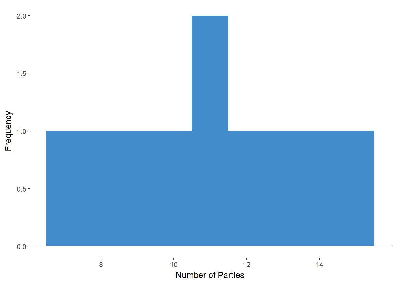 Figure 11.3. Histogram of Freshmen Party Count
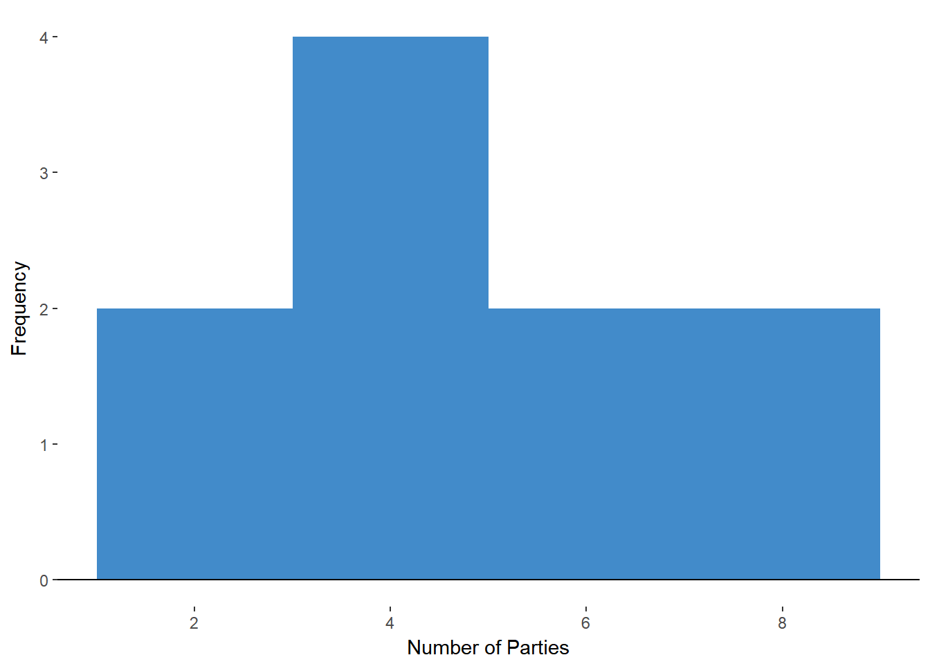
Figure 11.4 Histogram of Senior Party Count
- Random Sampling. This assumption is met according to the problem information.
- Independence of Observations. Given the random sampling, we believe this to be true.
- Equal variances. Let’s calculate our sample variances to determine if the ratio of large to small is less than 2.
Recall that variance is the average squared distance of each value from the mean \[ s^2 = \frac{\Sigma (X-M)^2}{n-1} \]
Using this formula we get \(s^2_{Freshmen}=6.67\) and \(s^2_{Seniors}=6.32\)
The ratio of large to small is 1.06, which is below our threshold of 2. Therefore, our assumption of equal variances can stand.
Statistical Hypotheses
Before we get to any calculations, we need to make our hypotheses explicit. The null hypothesis (H0) is that the two groups came from the same populations. Thus: \[ H_0 : M_{Freshman} = M_{Senior} = \mu_0 \] The alternative hypothesis is that the groups come from different populations. That is: \[ H_a : M_{Freshman} \neq M_{Senior} \neq \mu_0 \]
\(\alpha\)-level
Next, we need to establish the \(\alpha\)-level for the test of statistical significance. Per custom, let’s choose a two-tailed test at \(\alpha\) = 0.05. Because it is two-tailed, we’ll look for the critical value that is associated with a probability of 0.025.
Degrees of Freedom
Before we can find that critical value, we need to determine the degrees of freedom. Recall that the total degrees of freedom for a two independent-sampels t-test is N - 2. We have 20 individuals in our little survey so df = 20 - 2 = 18.
Critical Value
We can now find our critical value by looking at the intersection of the degrees of freedom (18) and the \(\alpha\)-level (0.025). The table gives a value of tcrit = 2.10.
T-value
We’ve got the easy stuff out of the way; now it is time to crunch some numbers. Let’s start with the general formula:
\[ t = \frac{M_{Freshman}-M_{Senior}}{S_{M_1-M_2}} \]
Before we can add any values to the formula, we will need the sample means for both freshmen and seniors. \[ \begin{aligned} M_{freshmen} &= \frac{(7 + 8 + 10 + 11 + 12 + 9 + 13 + 14 + 15 + 11)}{10} = 11 \\ \\ M_{seniors} &= \frac{(4 + 8 + 9 + 6 + 4 + 5 + 1 + 2 + 7 + 5)}{10} = 5.1 \end{aligned} \]
Our numerator thus becomes: \[ t = \frac{11 - 5.1}{S_{M_1-M_2}} = \frac{5.9}{S_{M_1-M_2}} \]
The next step is to calculated the standard error of the difference. Here is the formula once more:
Because we have equal sample sizes, we can use the reduced formula for the pooled variance: \[ s^2_p = \frac{s^2_1 + s^2_2}{2} \]
As calculated during our assumption checks, \(s^2_{Freshmen}=6.67\) and \(s^2_{Seniors}=6.32\)
Let’s plug those back into our equation for pooled variance: \[ s^2_p = \frac{s^2_1 + s^2_2}{2} = \frac{6.67 + 6.32}{2} = \frac{12.99}{2}=6.50 \]
We’re getting closer! Let’s plug that into our simplified equation for standard error of the difference for equal sample sizes.
\[ S_{{M_1}-{M_2}} = \sqrt{\frac{6.50}{10}+\frac{6.50}{10}}=1.14 \]
Finally, we can calculate the t-value:
\[ t = \frac{M_{freshmen}-M-{seniors}}{S_{M_1-M_2}} = \frac{5.9}{1.14} = 5.18 \]
Compare Calculated to Critical
To decide if we should reject the H0 that our two samples are derived from the same population, we need to determine if our calculated t-value is more extreme than our critical t-value. Because \[ \begin{aligned} t_{crit} & = 2.10 \\ & \text{and} \\ t_{calc} & = 5.18 \\ \\ t_{crit} & < t_{calc} \end{aligned} \] There for we should reject H0. Figure 11.5 places tcrit and tcalc on the t-distribution to highlight the decision making process.
Figure 11.2. Null Hypothesis Significance Testing with the T-Distribution
Confidence Interval.
Of course, no test is complete without calculating our confidence interval. For this example, we want a 95% confidence interval but we’ll have to update our interval limit equations to reflect the two independent-samples t-test. Here are the original equations: \[ \begin{aligned} CI_{upper} & = M + t_{crit}*\sigma_M \\ CI_{lower} & = M - t_{crit}*\sigma_M \end{aligned} \] We are no longer asking about a single mean. In our t-test, we incorporated the two means by finding the difference between them. We will use the difference of the two means in calculating the confidence interval.
We also need to update our standard error. In the one-sample version, we used the standard error of the mean. We’ll now need to use the standard error of the difference. Our new equations are thus: \[ \begin{aligned} CI_{upper} & = (M_1 - M_2) + t_{crit}*S_{M_1 - M_2} \\ CI_{lower} & = (M_1 - M_2) - t_{crit}*S_{M_1 - M_2} \end{aligned} \] Let’s plug in our values that we found or calculated earlier to find our 95% confidence interval. \[ \begin{aligned} CI_{upper} & = (M_1 - M_2) + t_{crit}*S_{M_1 - M_2} = 5.9 + 2.10*1.14 = 8.29 \\ CI_{lower} & = (M_1 - M_2) - t_{crit}*S_{M_1 - M_2} = 5.9 - 2.10*1.14 = 3.506 \end{aligned} \] Our 95% CI is [3.50, 8.29]. What does this mean again? First we need to remember that we are no longer representing a range of estimates for population means but rather the estimates for a difference between two population means. As such, we would report that 95 of 100 sets of two samples of size 10 would likely yield differences between the means of 3.50 and 8.29.
We can link this back to our NHST by determining if our H0 is included in the interval. Recall that our null hypothesis is that the two samples came from the same population and thus that there is no difference between the sample means. As such, we want to determine if 0 is included in the interval.
Because a mean difference of 0 is not included in [3.50, 8.29], we will reject H0.
Summing Up Two Independent-Samples T-Test
The two independent-samples t-test is a tool that allows us to judge if two independent groups differ. More specifically, we are determining the probability that two means came from the same population. To do this, we had to adjust our t-test to include the difference of sample means and a new standard error of the difference. Apart from a new assumption (equality of variance) and a few new values to calculate, the procedures for the two independent-samples t-test is identical to the one-sample t-test and the one-sample z-test.
The two sample-independent samples t-test is very helpful for many situations but it is not appropriate for when we want to know if two related groups are different. For this, we’ll need another adjustment.
Paired-Samples T-test
Just as we may want to know if two independent groups are different, we may also want to know if two related groups are different. Here are a few examples:
- Do individuals rate themselves as more tired after a lecture compared to before a lecture?
- Are fathers more fiscally conservative than their sons?
The first example would require a within-subjects design. That is, we would assess the the dependent variable in multiple conditions (i.e., levels of the independent variable) for each participant.
Within-subjects designs are also known as repeated-measures designs. The occur when multiple observations are made from each participant.
The second example would require a between-subjects design. That is, we would assess the dependent variable once for each participant because the participant only receives one level of the independent variable. This may be by design or natural occurrence. For example, a participant can only be the father or the son in the tested pairs in or example.
Between-subjects designs assess the dependent variable only once for each participant.
The key to both of these examples is that we believe there to be some relationship between the observations. That is, because the “tiredness” rating is coming twice from the same individual, we should assume that those ratings will be related. When the values are related, we will need the paired-samples t-test. This test is very similar, conceptually, to those we’ve performed before but requires a little pre-processing of the data. Rather than examine the difference of the means of two groups, we will compare the linked values first, then determine the mean of the differences. We’ll get into the details more in a minute. First, let’s check the procedure for using the test.
Steps for the Paired-Samples T-test
- Subtract paired values.
Subtract the second observation in the pair from the first observation in the pair for the complete data set.
- Determine the \(\alpha\)-level.
Are you performing a two-tailed test (please do!)? If so, divide \(\alpha\) by 2.
- Determine the df.
For one-sample t-test, df = n-1.
- Look up critical t-value.
Find at intersection of \(\alpha\) and df.
- Calculate t-value.
Use t-transformation formula.
- Compare calculated and critical t-values.
If calculated absolute value of t-value is greater than critical t-value, reject H0
- State conclusion.
Answer the research question given your decision regarding H0
As you may have noticed, these steps are equivalent to the one-sample t-test with an extra step at the beginning: subtract paired values. Here is a quick example of what that first step entails.
Subtracting Paired Value
For the paired-samples t-test, we are assuming that the observations are linked in pairs (e.g., before and after, relatives, matching on other qualities, etc.). As such, our presentation of the data will represent this pairing.
Table 11.2
Example of Paired Data
| Participant | Before | After |
|---|---|---|
| 1 | 0 | 5 |
| 2 | 3 | 4 |
| 3 | 2 | 2 |
We can easily perform the first step of subtracting values by adding another column to the right of the table that contains After - Before.
| Participant | Before | After | Difference |
|---|---|---|---|
| 1 | 0 | 5 | 5 |
| 2 | 3 | 4 | 1 |
| 3 | 2 | 2 | 0 |
The order of subtraction is not important as long as you consistently subtract in the same direction (e.g., Subtract before from after for all pairs). The resulting difference values will be the new sample on which we will bases our t-statistic. However, before we calculate that value, let’s state our assumptions.
Assumptions
Normality of population. Just as before, the population from which each sample is derived is assumed to be normally distributed.
Independence within groups. Although we are leaving behind total independence, we still need to assume that the values within a group (i.e., within a level of the independent variable) are independent. For example, the before scores should be independent of one another and the after scores should be independent of one another even though there is a link between before and after scores.
The Formula
The structure of the paired t-test formula is conceptually identical to the one-sample t-test, it just has some different symbols. \[ t = \frac{M_D - \mu_{D_0}}{S_{M_D}} \] In this formula, MD is the mean of the difference scores that we find in our first step. \(\mu_{D_0}\) is the null hypothesized mean of the difference scores. \(S_{M_D}\) is the Standard Error for Difference Scores. We’ll see ho we get each of these values. starting with \(\mu_{D_0}\)
The null hypothesis
In the verbal description, the null hypothesis is there is no difference between the groups. If the groups are assumed to be equal (i.e., from the same population) then the differences between the pairs should be, on average, zero. Our value for \(\mu_{D_0}\) is 0.
The numerator
The numerator for the t-tests is the difference between our sample and the hypothesized value. Because our hypothesized value (\(\mu_{D_0}\)) is 0, our numerator simply becomes the mean of the differences (MD).
To determine MD, we simply calculate the mean of the scores that result from subtracting the paired values. That is.
\[ M_D = \frac{\Sigma X_D}{n_D} \]
where xD is a difference score and nD is the number of difference scores.
Standard Error
Calculating the standard error of the difference scores is equivalent to the standard error of the mean from the one-sample t-test but is based off of the sample of difference scores. That means that we need to find the standard deviation of the sample of difference scores then divide by the square root of the number of difference scores.
\[ S_{M_D} = \frac{S_D}{\sqrt{n_D}} \]
This value tells us how far each mean difference is from the population mean difference, on average.
Degrees of Freedom
The parallels with the one-sample t-test follow for the degrees of freedom. Recall that we had N-1 degrees of freedom for the one-sample t-test. For the paired-samples t-test, we will have nD-1 degrees of freedom.
But we have two groups! Why don’t we subtract a degree of freedom for each group? We are only losing 1 degree of freedom because we are only estimating one population mean: the population mean difference. Because we combined the two samples into one by subtraction, we are now only working with one sample mean difference and one population mean difference.
**Degrees of freedom for the paired-samples t-test* are equal to the number of difference scores minus 1 or nD - 1.
Let’s walk through an example for the paired-samples t-test.
Example
You’ve recently written a self-help book that claims to increase life satisfaction for those that follow the steps. Your publisher asks 11 randomly selected people to read the book and try out the steps. She records ratings of life satisfaction (0 = extremely dissatisfied, 100 = extremely satisfied) before reading the book and 3 months after starting to practice the steps. Here are the data:
| Participant | Before | After |
|---|---|---|
| 1 | 39 | 45 |
| 2 | 41 | 46 |
| 3 | 42 | 48 |
| 4 | 42 | 49 |
| 5 | 46 | 49 |
| 6 | 47 | 49 |
| 7 | 49 | 49 |
| 8 | 50 | 51 |
| 9 | 52 | 51 |
| 10 | 53 | 53 |
| 11 | 55 | 55 |
Check Assumptions We’ll check our assumption of normality by assessing the histograms. Figures 11.6 and 11.7 are histograms for the “before” and “after” samples respectively.
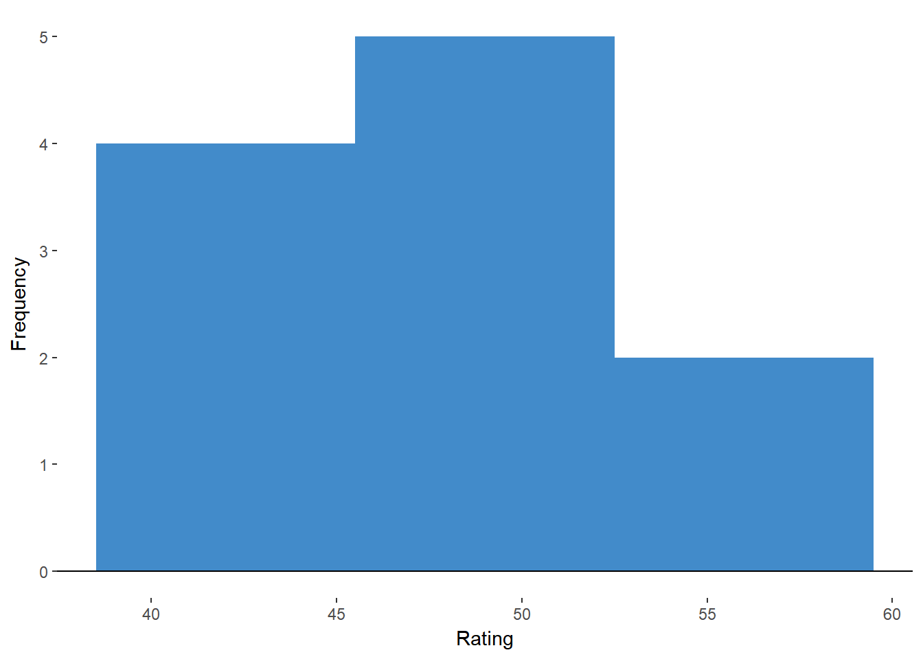
Figure 11.6. Histogram of Before Ratings.
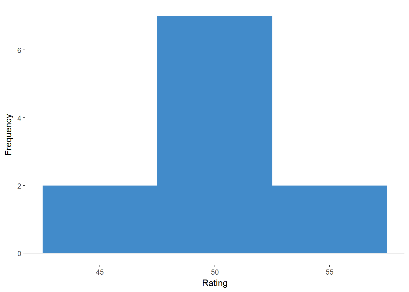
FIgure 11.7 Histogram of After Ratings.
These look roughly normal enough for us to maintain this assumption.
The assumption of independence within group (no relationship between participants) is valid because of the random sampling.
Step 1. Subtract paired values We’ll find the difference scores by subtracting the before from the after.
| Participant | Before | After | Difference |
|---|---|---|---|
| 1 | 39 | 45 | 6 |
| 2 | 41 | 46 | 5 |
| 3 | 42 | 48 | 6 |
| 4 | 42 | 49 | 7 |
| 5 | 46 | 49 | 3 |
| 6 | 47 | 49 | 2 |
| 7 | 49 | 49 | 0 |
| 8 | 50 | 51 | 1 |
| 9 | 52 | 51 | -1 |
| 10 | 53 | 53 | 0 |
| 11 | 55 | 55 | 0 |
Step 2. Determine the \(\alpha\)-level We’ll stay tried-and-true with the two-tailed test at \(\alpha\) = 0.05
Step 3. Determine the df
For one-sample t-test, df = n-1. For the paired-samples t-test, df=nD - 1. We have 11 pairs so we have 11 - 1 = 10 degrees of freedom.
Step 4. Look up critical t-value With df = 10 and a two-tailed \(\alpha\)-level of 0.05, we’ll look for the critical value at the intersection of df = 10 and \(\alpha\) = 0.025. The table gives us a critical t-value of 2.23.
Step 5. Calculate t-value
Our formula for the paired-samples is \[
t = \frac{M_D}{S_{M_D}}
\]
We’ll need to calculate the mean of the differences for the numerator. \[ M_D = \frac{\Sigma X_D}{n_D} = \frac{(6 + 5 + 6 + 7 + 3 + 2 + 0 + 1 + -1 + 0 + 0)}{11} = 2.64 \]
We’ll also need our sample standard deviation in order to calculate the standard error of the difference scores.
\[ S_D = \sqrt{\frac{\Sigma (X_D - M_D)^2}{n_D - 1}} = 2.91 \]
The standard error of the difference scores is thus:
\[ S_{M_D} = \frac{S_D}{\sqrt{n_D}} = \frac{2.91}{\sqrt{11}} = 0.88 \]
With both our numerator and denominator calculated, we can find our t-value.
\[ t = \frac{M_D}{S_{M_D}} = \frac{2.64}{0.88} = 3.00 \]
Step 6. Compare calculated and critical t-values Our tcrit = 2.23 and the tcalc = 3.00. We will reject H0 that the before and after scores came from the same population.
Step 7. State conclusion The individuals had higher life satisfaction after reading the book and following the steps than before reading the book.
Confidence Interval How much of a difference from before to after might we expect in the larger population? A confidence interval can give us that information. We’ll have to update our previous formulas quickly before we continue. \[ \begin{aligned} CI_{upper} & = M + t_{crit}*\sigma_M \\ CI_{lower} & = M - t_{crit}*\sigma_M \end{aligned} \] These limits for the one-sample t-test can easily be amended to ft the paired-samples t-test by substituting difference score equivalents for the single sample information. \[ \begin{aligned} CI_{upper} & = M_D + t_{crit}*S_{M_D} \\ CI_{lower} & = M_D - t_{crit}*S_{M_D} \end{aligned} \] Now let’s plug in our values to find our limits. \[ \begin{aligned} CI_{upper} & = M_D + t_{crit}*S_{M_D} = 2.64 + 2.33*0.88 = 4.69\\ CI_{lower} & = M_D - t_{crit}*S_{M_D} = 2.64 - 2.33*0.88 = 0.59 \end{aligned} \] Notice that \(\mu_{D_0}\) = 0 is not included in our interval so we would have the same decision regarding H0. The 95% CI informs us that most samples would yield a pre-post difference of 0.59 to 4.69.
Summing Up Paired-Samples T-test
The paired-samples t-test allows us to judge if two related samples are different. That is, we can decide if within-subjects or matched-pairs data came from the same population. In combination with the other t-tests, we can make inferences for a range of situations.
Summing up T-Tests
The t-tests and associated t-distributions are based on the z-test and standard normal distribution. They have been altered to include the possibility of error derived from estimating a population variance from a sample. The smaller the sample, the fewer the degrees of freedom and the less certainty we have in our estimate. This uncertainty is represented in wider t-distributions and larger critical values. Although it may require a larger effect to reject H0 for a t-test with small to moderate sample size than for a z-test, we can be more confident that we are avoiding the dreaded Type I Error.
Where We’re Going
The family of t-tests were a wonderful development. Unfortunately, the t-tests are limited to comparing two samples at most. There are many situations in which it would be beneficial to compare multiple groups. For example, perhaps we have reason to believe that hair color has some implication for perceived friendliness. If we were to use the t-test approach, we would have to calculate a t-test for Blonde vs. Brunette, Blonde vs. Red, Blonde vs. Black, Brunette vs Red, Brunette vs. Black, Red vs. Black, … and we haven’t even gotten into the artificial colors! This would be a lot of t-test. A part from the burden of all of these calculations, we have to be aware of the possibility of all the errors in these tests. In the next section, we’ll explore the Analysis of Variance (ANOVA) approach to dealing with multiple comparisons.
Try out your understanding of the family of t-tests by completing and submitting the homework before you take the quiz.