By completing this section, you will be able to
- Explain the need for Analysis of Variance in addition to the t-test
- Describe the null and alternative hypotheses for ANOVA
- List the assumptions of ANOVA
- Find critical values in the F-table
- Identify the different sources of variance
- Calculate sums of squares
- Calculate the F-statistic for the one-way ANOVA
Professor Weaver’s Take
Do you like vegetables? I do. I am particularly fond of fresh corn on the cob in the summer. Have you ever heard that corn should be knee-high by the fourth of July? It seems that it is always taller than that by early July. I think that corn grows so big so quickly because of statistics. In particular, I credit the Analysis of Variance. Before you get to concerned about my health, let me give you some context.
The statistician Sir Ronald Fisher (yes, he was knighted for his statistical work) developed techniques to help understand how various factors influenced plants. The Analysis of Variance was used with the split-plot design in which a plot of land was divided into several sections onto which different treatments were applied to plants. The statistics analysis allowed researchers to determine how each factor differed from the others. This greatly improved the speed and efficiency of crop research.
See? Vegetables are better because of statistical knights!
Cheekiness aside, Fisher’s work is useful in many designs and applications outside of crops. We’ll be generalizing our understanding of group differences that we established with the t-tests.
When T Is Not Enough
The t-test is great! We learned how to incorporate the uncertainty of having to estimate population standard deviation into our tests and how to judge the similarity of two groups. With this technique, we could answer any questions regarding to group differences. Unfortunately, to use the t-test to compare multiple groups can lead to a few issues
- For every comparison, we would need a t-test. For 10 groups, we would need 45 t-tests to compare all of the groups
- We increase the likelihood of having a Type I error for each test.
When we set \(\alpha\) = 0.05, we are saying that we are OK with 1 out of every 20 tests yielding a false positive. If we do 45 there’s, were expecting 2 to give a false positives. This is not an acceptable way to test hypotheses! We need a way to compare more than 2 groups without drastically increasing the family-wise error rate.
Family-wise Error Rate is the probability of making a type I error in all of the tests performed.
Generalizing the T-Test
Let’s work from the two independent-samples t-test. Here’s the formula:
\[t = \frac{M_1-M_2}{S_{M_1-M_2}}\]
The numerator represents the effect by finding the distance between the group means. The denominator represents the error by finding average distance each score is from that group’s mean.
Comparing Multiple Means
It is easy to find the difference between two means, we simply subtract one from the other. How can we find the difference among three means? Serial subtraction won’t work. The more means we add, the further negative the difference becomes. What we need is a way to summarize how different the means are. Wait a minute… I think this sounds a lot like the standard error of the mean. That’s summarized how different each possible sample mean was from the population mean. We’ll be using the same logic to assess how different our dance means are.
Error
To explain why the variance or average distance of scores from means is considered error, we need to remember that the mean is the best guess for the population value. That is, we expect to find just the population value and when we get scores that differ from that, we consider that to be an error in our statistical model. We’re not saying that an individual’s response is wrong, we just mean that our model cannot explain why that score is different. We are incorporating the group to which a score belongs into the numerator so we expect the scores between groups to be different. We don’t know, however, why the scores within the the groups should vary. This unexplained variance becomes the error variance in our Analysis of Variance.
Analyis of Variance (ANOVA): General Overview
The One-Way Between-Subjects ANOVA, so called because it examines only one independent variable with levels applied to different groups. allows us to compare multiple means without increasing the chances of Type I errors. We can do this by determining if the variability of the group means is greater than the variability of individual scores within the group. That is, we find the ratio of the variability due to the effect (i.e., the change in the independent variable) to the variability of scores due to error (i.e., within-group variability). If the ratio is large enough, we can claim that at least one of the means is statistically significantly different from another. We’ll have to perform some extra steps to parse out the significant means after we find a significant F-statistic.
Here is the formula for the Between-Subjects ANOVA:
\[F = \frac{\text{MS}_{\text{Between}}}{\text{MS}_{\text{Within}}}\]
We are fiding an F-statistic that corresponds to values in an F-distribution. MS stands for mean square and it is very similar to variance.
\[\text{MS}=\frac{\text{Sum of Squares}}{df}\]
The sums of squares are the first few steps of calculating variance in which you find the difference between a score and a mean, sqaure those differences, then add up all of the squared scores.
The degrees of freedom are determined in the same way as the t-test. Take the number of values and subtract the number of estimated population means. We’ll get into more details about this soon.
Sources of Variation
The one-way ANOVA partitions the total variance into two sources: the variance due to the effect and error variance. This division and associated components are represented in the ANOVA table.
Table 12.1
The ANOVA Table
| Source | SS | df | MS | F |
|---|---|---|---|---|
| Between | \(\Sigma n(M_k-GM)^2\) | k-1 | \(\frac{\text{SS}_{\text{Between}}}{df_{\text{Between}}}\) | \(\frac{\text{MS}_{\text{Between}}}{\text{MS}_{\text{Within}}}\) |
| Within | \(\Sigma (X-M_k)^2\) | N-k | \(\frac{\text{SS}_{\text{Within}}}{df_{\text{Within}}}\) | - |
| Total | \(\Sigma (X-GM)^2\) | N-1 | - | - |
As you calculate the Analysis of Variance, you can fill in the values using these equations to keep track of the components.
Before we get into transforming the equations into steps, let’s examine the assumptions of ANOVA and then the statistical hypotheses to determine how they map onto these sources of variance.
Assumptions of the Between-Subjects ANOVA
Categorical independent variable
The levels of the independent variable should differ by kind rather than amount.
Interval/Ratio scale for dependent variable
To be able to determine means and variances, we will need a scale of measurement for which the mean and variance are appropriate (i.e., interval or ratio scales).
Normally distributed dependent variable (within each group)
With the heavy use of mean and variance, we must have normally distributed data for those statistics to be valid representations of the central tendency and variability.
Independent observations within and between groups
The scores within one group should not be related and the scores between the groups should not be related. If this assumption is violated (e.g., the same person gives responses to multiple levels), you’ll need to take a different approach (E.g., a Within-Subjects ANOVA)
Homogeneity of variance (equal variance across groups)
Lastly, to ensure that we have modeled the error correctly, we need to be sure that the variance within each group is roughly equal. If the groups do not have roughly equal variance (no group with twice the variance of another), the degrees of freedom need to be adjusted. This adjustment is often done with statistical software.
The Null Hypotheses
In general, the null hypothesis is that there is no effect of a variable on another variable. For the independent-samples t-test and the between-subjects ANOVA, our null hypothesis (\(H_0\)) is that there is no difference between the group means. If all of the group means are equal we would expect zero variability among those means. That is, \(SS_{\text{Between}}\) should equal zero.
The null hypothesis for the one-way between-subjects ANOVA is \(H_0: M_1 = M_2 = ... = M_k\)
If the variability is greater than zero, should we reject \(H_0\)? Similar to the two independent-samples t-test, we can have a numerator that is not zero and still fail to reject \(H_0\). The decision to reject \(H_0\) depends on different the means are relative to how much random variability we would expect if \(H_0\) were true. Just as with the t-tests, we can make this judgement by consulting a table or critical values.
The F-Table
The F-Table contains the critical F-values corresponding to \(\alpha\) = 0.05 and \(\alpha\) = 0.01 for the F-distribution with degrees of freedom \(df_1\) and \(df_2\).
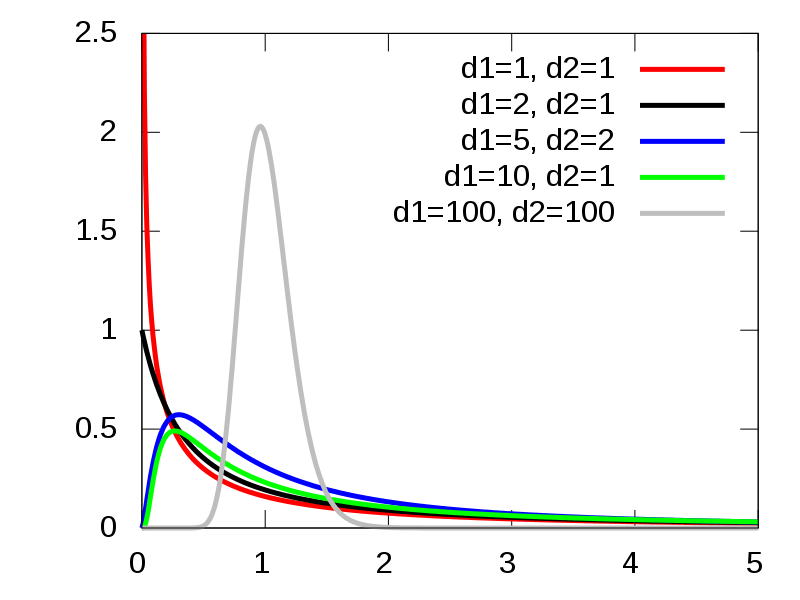
F Distributions
Figure 12.1 A few F-dsitributions. Reproduced from https://en.wikipedia.org/wiki/F-distribution.
The first \(df\) refers to the between-subjects degrees of freedom adn \(df_2\) refers to the within-subjects degrees of freedom. Here is an excerpt from the table.
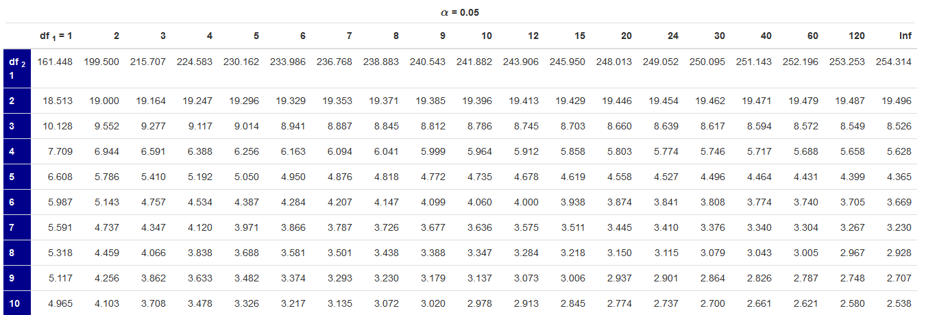
F Table
Figure 12.2. Excerpt of F-table
Notice how there are only positive values in the table. This is not just to reduce redudnency as in the normal and t-distributions. There are no negative F-values. Why is that? Recall that the F-value is a ratio of two variances and that variances are average sums of squares. The key is that we are dealing with squared values, which are always positive. Therefore, any division will also result in positive values. The real impact for null hypotheis significance testing (NHST) is that we will always perform a one-tailed test. That is, we will always look for a critical value associated with \(\alpha\) rather than a two tailed test that has a critical value associated with \(\frac{\alpha}{2}\).
Also motice how the critical values get smaller as the within-subjects degrees of freedom increase. This means, just like the t-tests, our statistical power will increase as we increase sample size. The critical values get larger as the between-subjects degrees of freedom increases. That is, as we add more groups, we need more evidence to argue that they are not all equal.
Decision Regarding \(H_0\)
Just as we had with the one-sample z-test and the family t-tests, we will decide to reject \(H_0\) if \(F_{calc} > F_{crit}\). Remember that when the calcualted statistic is more extreme than the critical statistic, it suggest that the probability of making a Type I Error (false positive) is less than \(\alpha\).
If we are only comparing two means (the equivalent of the two independent-samples t-test), we stop at the F-statistic as that will tell us that the two sample means are likely from two different populations. For most ANOVA applications, however, we want to compare more than two samples. In these cases, a significant F-test (i.e., we reject \(H_0\)) leaves some ambiguity. We know that there is atleast one mean that is statistically significantly different from the others but we don’t know which means are different. When the number of groups (k) is greater than 2 and \(H_0\) is rejected, you must perform post-hoc analyses to determine which means differ.
Post-Hoc Analyses
Post-hoc means “after the fact.” These are follow up tests we perform to determine which of the means are statistically different following a significant ANOVA. In these post-hoc analyses, we will decide if the difference between each possible pair of means is statistically significantly different. Now that we are only comparing two means at a time, we can perform a version of a t-test. Although there are various versions, I recommend Tukey’s Honestly Significant Difference (HSD) test befcause it is less likely to make a Type I Error than other versions.
Tukey’s Honestly Significant Difference (HSD) Test
There are three general steps to the Tukey HSD.
- Find the differences for each possible pair of means.
- Calculate the critical difference.
- Decide which means have a difference greater than the critical difference.
STEP 1: Once you’ve calculated the sample means for your ANOVA, you’ll need to determine all of the ways those means may be put into pairs. If you have three means, you would have the following comparisons:
A - B
A - C
B - C
If you had four means, you would have the following comparisons:
A - B
A - C
A - D
B - C
B - D
C - D
You can easily find the total number of comparisons by using the combinations formula:
\[\frac{N!}{n!(N-n)!}\]
If we had 5 means, we would have:
\[\frac{N!}{n!(N-n)!}=\frac{5!}{2!(5-2)!}=\frac{5\times4\times3\times2\times1}{(2\times1)(3\times2\times1)}=\frac{120}{12}=10\]
NOTE: If you do have many different levels of an independent variable, it is possible that those levels may start to approach an ordinal or interval scale. If that is the case, you may want to consider an alternative modeling technique such as linear regression.
Once you have established all of the pairwise comparisons, simply find the difference between the means. It will also be helpful if you order the values from smallest to largest.
STEP 2: To determine if any of those differences are statistically significantly different, we need a critical value. The critical value is found using the following formula:
\[q_{\alpha}\sqrt{\frac{\text{MS}_{\text{Within}}}{n}}\]
We get \(\text{MS}_{\text{Within}}\) from the ANOVA table, n is the number of observations per group, and \(q_{\alpha}\) comes from the Studentized Range Table. Figure 12.3 shows an excerpt from this table.
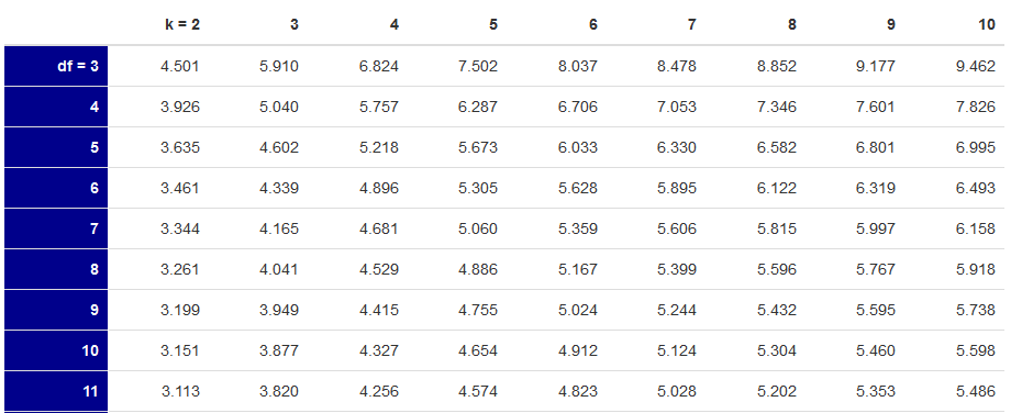
Q Table
Figure 12.3 Excerpt from Studentized Range Table
To find the appropriate \(q_{\alpha}\), you’ll need the \(df_{\text{Within}}\) and the number of groups (k).
Plug all of the values into the critical value equation to find minimum distance needed for two means to be statistically significantly different.
STEP 3: If you’ve ordered the differences from largest to smallest, it will be easy to find which comparisons are larger than the critical difference. Any difference that is larger than the critical difference is considered a statistically significant difference.
We’ll walk through these steps again with a full example.
Summing Up ANOVA in General
The Analysis of Variance (ANOVA) approach is used to determine if multiple samples are from the same population. Rather than perform multiple t-tests which can increase our family-wise type I error rate, we examine all of the means at once by calculating the variability of the sample means. To determine if there is a statistically significant difference among some of the means, we’ll compare the variability of the sample means to the variability within the samples.
If we reject the null hypothesis that all of the sample means are equal, we’ll perform post-hoc analyses. These post hoc analyses determine if the difference between means is larger than expected by chance variation. We can perform these multiple tests because we have already detected a difference in the ANOVA where we controlled for type I error.
Calculating the F-statistic
Let’s restate the ANOVA table from earlier to help us determine the values we need to determine.
Table 12.1
The ANOVA Table
| Source | SS | df | MS | F |
|---|---|---|---|---|
| Between | \(\Sigma n(M_k-GM)^2\) | k-1 | \(\frac{\text{SS}_{\text{Between}}}{df_{\text{Between}}}\) | \(\frac{\text{MS}_{\text{Between}}}{\text{MS}_{\text{Within}}}\) |
| Within | \(\Sigma (X-M_k)^2\) | N-k | \(\frac{\text{SS}_{\text{Within}}}{df_{\text{Within}}}\) | - |
| Total | \(\Sigma (X-GM)^2\) | N-1 | - | - |
To be able to calculate the F-statistic, we’ll need:
- Group Means (\(M_k\))
- Grand Mean (GM)
- Sum of Squares - Between (\(\text{SS}_{\text{Between}}\))
- Degrees of Freedom - Between (\(df_{\text{Between}}\))
- Sum of Squares - Total (\(\text{SS}_{\text{Total}}\))
- Degrees of Freedom - Total (\(df_{\text{Total}}\))
That’s all!
Okay, it is still a long list but we left out a few. We will not have to directly calculate the Sums of Squares - Within or the associated degrees of freedom. We can forego these steps because \(\text{SS}_{\text{Within}}=\text{SS}_{\text{Total}} - \text{SS}_{\text{Betweem}}\). If we have the formulae for all of the sums of squares, why should we pick those for Between and Total? I choose those because I’m lazy. It is easier to calculate the total sums of squares and subtract away the between than it is to calculate the sums of squares within.
Once we have all of these components, we can complete our ANOVA table to determine our F-statistic. We can then compare that to the appropriate critical value from the F-table. If we can reject \(H_0\), we’ll perform Tukey’s HSD test to determine which means are statistically significantly different from one another.
Let’s walk through a full example:
Example
Imagine that you are a political adviser for presidential candidates. You have a theory that the color of shirt one wears for a debate influences positive ratings from viewers. You tell your candidate to choose her shirt color carefully but she isn’t convinced. You haven’t verified this yourself so you decide to collect some data to put your theory to the test. You ask thirty students to watch videos of candidates giving a prepared speech then indicate their rating of the candidate on a scale from 0 (Extremely Negative) to 100 (Extremely Postive).
Ten randomly selected students watched a candidate wearing a blue shirt, another ten randomly selected students watched a candidate wearing a white shirt, and another ten randomly selected students watched a cadidate wearing a red shirt. Importantly, all students actually saw the same candidate giving the same speech so that the only aspect that varied was the color of shirt. Each student watched the video by him or herself.
Here are the data:
| Blue | White | Red |
|---|---|---|
| 86 | 58 | 35 |
| 81 | 52 | 44 |
| 79 | 67 | 29 |
| 82 | 77 | 31 |
| 73 | 65 | 26 |
| 72 | 60 | 28 |
| 69 | 69 | 40 |
| 64 | 70 | 30 |
| 60 | 74 | 24 |
| 58 | 49 | 29 |
Assumptions
Categorical independent variable
The independent variable is color of shirt, which is definitely categorical.
Interval/Ratio scale for dependent variable
Our dependent variable is rating. This variable has a 0 and even spacing between the scores so it appears to be ratio. However, the 0 is arbitrary as we could easily have made “extremely negative” equal to -50. Does this make this an interval scale? We are safe to assume interval scale but it is hard to argue that everyone has the same understanding of how a rating of 48 and 49 differ.
Normally distributed dependent variable (within each group)
We can check this a number of ways. We can look at the histograms which are shown below. We can compare the mean, median, and mode for congruence, or we can calculate the skew for each distribution. The latter requires some calculations that are beyond the scope of this book but that appraoach is the prefered method when using statistical software.
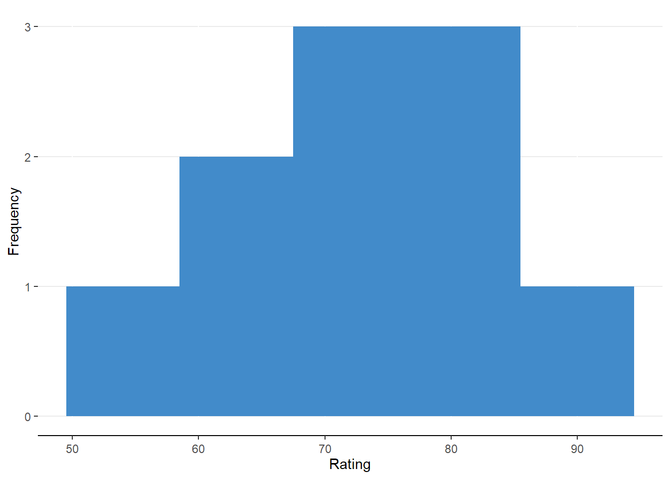 Figure 12.4. Histogram for Rating of Candidate Wearing Blue Shirt
 Figure 12.5. Histogram for Rating of Candidate Wearing White Shirt
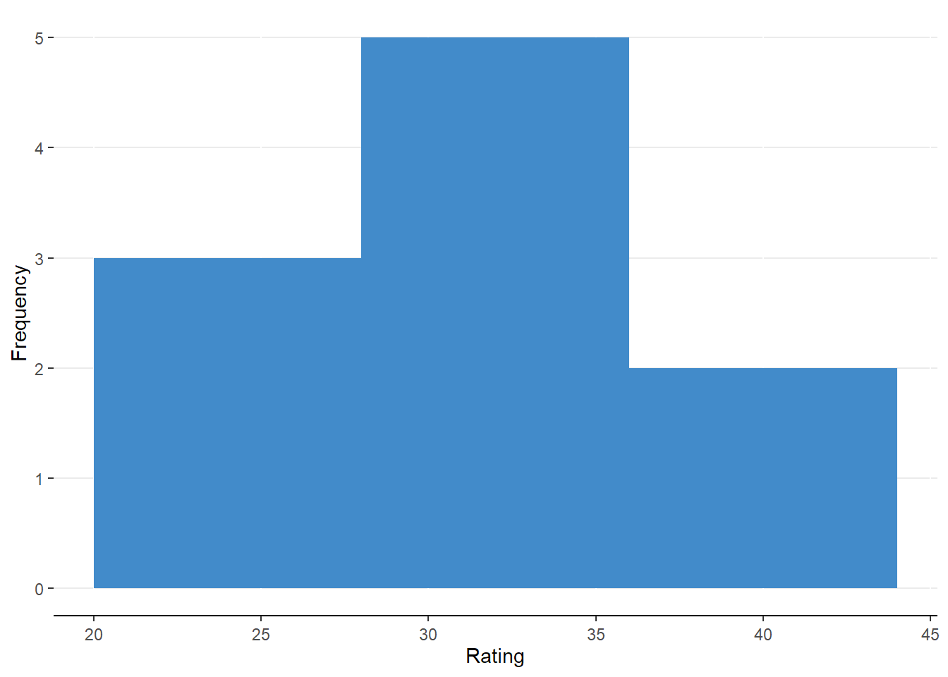 Figure 12.6. Histogram for Rating of Candidate Wearing Red Shirt
The histograms suggest a roughly normal distribution for each group of ratings.
Independent observations within and between groups
We can maintain this assumption because of the description but we could test it more formally with an analysis of correlated errors. That analysis is much more tenable with software packages than by hand.
Homogeneity of variance (equal variance across groups)
We’ll have to save this assumption for when we start calcualting values for our ANOVA table.
Group Means
Now that we’ve check (almost) all the assumptions, we can determine the mean for each group.
\[M_{Blue} = \frac{86+81+79+82+73+72+69+64+60+58}{10}=72.4\] \[M_{White} = \frac{58+52+67+77+65+60+69+70+74+49}{10}=64.1\] \[M_{Red} = \frac{35+44+29+31+26+28+40+30+24+29}{10}=31.6\]
We’ll be using these for determining our between groups sums of squares
Grand Mean
The grand mean is the “mean of all means.” Literally, it is. To find the grand mean, you simply take the mean of the group means.
\[GM = \frac{M_{Blue} + M_{White} + M_{Red}}{k}=\frac{72.4+64.1+31.6}{3}=\frac{178.1}{3}=56.03\]
Sums of Squares
With our means calculated, we can find the between-groups sums of squares and the total sums of squares.
Between-Groups Sum of Squares The ANOVA table contains the formula:
\[\text{SS}_\text{Between}=\Sigma n_k(M_k - GM)^2\]
We can turn this into a step by step procedure by following PEMDAS.
- Subtract the GM from sample mean.
- Square each difference score
- Multiply each difference score by the number of observations within the corresponding groups.
- Add up all of the products.
Let’s put this into action
\[ \begin{aligned} \text{SS}_\text{Between}=\Sigma n_k(M_k - GM)^2 &= n_{\text{Blue}}(M_{\text{Blue}}-GM)^2 + n_{\text{White}}(M_{\text{White}}-GM)^2 + n_{\text{Red}}(M_{\text{Red}}-GM)^2\\ &=10(72.4-56.03)^2+10(64.1-56.03)^2+10(31.6-56.03)^2 \\ &=10\times16.37^2 + 10\times8.07^2 + 10\times-24.43^2 \\ &=10\times267.98 + 10\times65.12 + 10\times596.82 \\ &=2679.8 + 651.2 + 5968.2 \\ &=9299.2 \end{aligned} \]
Let’s update the ANOVA table with the new information
Table 12.2
Updated ANOVA Table
| Source | SS | df | MS | F |
|---|---|---|---|---|
| Between | 9299.2 | k-1 | \(\frac{\text{SS}_{\text{Between}}}{df_{\text{Between}}}\) | \(\frac{\text{MS}_{\text{Between}}}{\text{MS}_{\text{Within}}}\) |
| Within | \(\Sigma (X-M_k)^2\) | N-k | \(\frac{\text{SS}_{\text{Within}}}{df_{\text{Within}}}\) | - |
| Total | \(\Sigma (X-GM)^2\) | N-1 | - | - |
Total Sum of Squares
The total sum of squares is easy to find but can be tedious at time. To determine \(\text{SS}_{\text{Total}}\), we need follow the equation:
\[ \Sigma (X-GM)^2 \]
In procedural steps, we need to:
- Find the difference between each score and the grand mean
- Square each difference score
- Add up all the squared scores
In our case
\[ \begin{aligned} \text{SS}_{\text{Total}} = \Sigma (X-GM)^2 &= (86-56.03)^2+(81-56.03)^2 + \dots +(35-56.03)^2 + (44-56.03)^2 + \dots + (58-56.03)^2 + (52-56.03)^2 \\ &= 898.20 + 623.50 + \dots + 442.26 + 144.72 + \dots + 3.88 + 16.24 \\ &= 11252.97 \end{aligned} \]
We’ll update the table again
Table 12.3
Updated ANOVA Table
| Source | SS | df | MS | F |
|---|---|---|---|---|
| Between | 9299.2 | k-1 | \(\frac{\text{SS}_{\text{Between}}}{df_{\text{Between}}}\) | \(\frac{\text{MS}_{\text{Between}}}{\text{MS}_{\text{Within}}}\) |
| Within | \(\Sigma (X-M_k)^2\) | N-k | \(\frac{\text{SS}_{\text{Within}}}{df_{\text{Within}}}\) | - |
| Total | 11252.97 | N-1 | - | - |
Within-Groups Sum of Squares
The remaining SS is easily found by simply subtracting \(\text{SS}_{\text{Between}}\) from \(\text{SS}_{\text{Total}}\)
\[ \begin{aligned} \text{SS}_{\text{Within}} &= \text{SS}_{\text{Total}} - \text{SS}_{\text{Between}} \\ &= 11252.97 - 9299.2 = 1953.77 \\ \end{aligned} \]
The updated table with complete Sums of Squares is below
Table 12.3
Updated ANOVA Table
| Source | SS | df | MS | F |
|---|---|---|---|---|
| Between | 9299.2 | k-1 | \(\frac{\text{SS}_{\text{Between}}}{df_{\text{Between}}}\) | \(\frac{\text{MS}_{\text{Between}}}{\text{MS}_{\text{Within}}}\) |
| Within | 1953.77 | N-k | \(\frac{\text{SS}_{\text{Within}}}{df_{\text{Within}}}\) | - |
| Total | 11252.97 | N-1 | - | - |
Believe it or not but the hard part is done! The rest is simple calculation given numbers we already have.
Degrees of Freedom
The degrees of freedom are important for establishing our variances. Here are the formulas: \[ \begin{aligned} df_{Between} &= k - 1 = 3 -1 = 2 \\ df_{Within} &= N-k = 30-3 = 27 \\ df_{Total} &= N-1 = 30 - 1 = 29 \end{aligned} \]
We’ll quickly put those values in the table
Table 12.4
Updated ANOVA Table
| Source | SS | df | MS | F |
|---|---|---|---|---|
| Between | 9299.2 | 2 | \(\frac{\text{SS}_{\text{Between}}}{df_{\text{Between}}}\) | \(\frac{\text{MS}_{\text{Between}}}{\text{MS}_{\text{Within}}}\) |
| Within | 1953.77 | 27 | \(\frac{\text{SS}_{\text{Within}}}{df_{\text{Within}}}\) | - |
| Total | 11252.97 | 29 | - | - |
Mean Squares
We’ll use the first two columns to determine the values of the mean squares, Simply divide the SS by the df.
\[ \begin{aligned} MS_{Between} = \frac{\text{SS}_{\text{Between}}}{df_{\text{Between}}} = \frac{9299.2}{2} = 4649.6 \\ MS_{Within} = \frac{\text{SS}_{\text{Within}}}{df_{\text{Within}}} = \frac{1953.77}{27} = 72.36 \end{aligned} \]
Into the table go our new values.
Table 12.5
Updated ANOVA Table
| Source | SS | df | MS | F |
|---|---|---|---|---|
| Between | 9299.2 | 2 | 4649.6 | \(\frac{\text{MS}_{\text{Between}}}{\text{MS}_{\text{Within}}}\) |
| Within | 1953.77 | 27 | 72.36 | - |
| Total | 11252.97 | 29 | - | - |
The last step is to find the F-statistic
F-statistic
We’ll follow through with division for the last step of calculation.
\[ F = \frac{\text{MS}_{\text{Between}}}{\text{MS}_{\text{Within}}} = \frac{4649.6}{72.36} = 64.26 \]
Our completed ANOVA table is thus:
Table 12.6
Completed ANOVA Table
| Source | SS | df | MS | F |
|---|---|---|---|---|
| Between | 9299.2 | 2 | 4649.6 | 64.26 |
| Within | 1953.77 | 27 | 72.36 | - |
| Total | 11252.97 | 29 | - | - |
Now that we have our calculated F-statistic, we need to determine the critical F-value.
Critical F-Value
We will find this value in the F-table with \(df_1\) = 2 and \(df_2\) = 27.
The table gives us a critical value of 3.354.
Decision Regarding \(H_0\)
Given that our obtained F-statistic is 64.26 and the critical F-value is 3.354, we should decide to reject \(H_0\). Although we can say with some certainty that the color of shirt influences ratings. We can not say which shirt(s) was is different from others without Tukey HSD
Post-hoc Analyses (Tukey HSD)
With Tukey’s Honestly Significant Difference test, we will be able to say if the distance between a pair of means is large enough to constitute a statistically significant change.
Find Differences The first step of Tukey HSD is to find the distance between the different means. In our example:
\[ \begin{aligned} M_{Blue} - M_{red} &= 72.5 - 31.6 = 40.9\\ M_{Red} - M_{White} &= 31.6 - 64.1 = -32.5\\ M_{Blue} - M_{White} &= 72.4 -64.1 = 8.3 \end{aligned} \]
Find Critical q-value
The Q-table list critical values associated with the degrees of freedom for the within-groups SS and the number of groups (k).From our ANOVA table, we find the \(df_{win}\) = 27 and \(k\)=3, The critical q for this example is thus: 3.506.
Calculate Critical Difference
We’ll now take that critical value of q and multiply it by a standard error of sorts: \[ q_{\alpha}\sqrt{\frac{\text{MS}_{\text{within}}}{n}}=3.35\times{\sqrt{\frac{72.36}{10}}} = 3.35\times\sqrt{7.236}=3.35\times2.69=9.01 \]
Compare Values
Are any of the mean difference scores greater than the critical difference?
\[ \begin{aligned} M_{Blue} - M_{red} &= 40.9\\ M_{white} - M_{red} &= 32.5\\ M_{Blue} - M_{White} &= 8.3 \end{aligned} \] All but the comparison between Blue shirt and White shirt was statistically significant because the differences of 8.3 is smaller than the critical difference of 9.01.
Conclusion
The significant F-test suggested that the color of shirt did impact ratings for a candidate during a speech. Post-hoc Tukey HSD test revealed that there were statistically reliable differences between the red shirt and the blue shirt, and between the white shirt and red shirt. That is, a candidate who wears a blue or white shirt are likely to be rated higher than a candidate with a red shirt.
Summing up One-Way Between-Subjects ANOVA
The one-way between-subjects ANOVA is a great tool for comparing multiple groups without increasing the family-wise type I error rate. We can do this by examining how the group means differ from one another relative to the variability of scores within groups. Should we find the ratio sufficiently large, we can reject the null hypothesis that the samples are equal.This will only tell us that atleast one of the means is different from the others. To disambiguate the difference among means, one should conduct the Tukey HSD test.
Where We’re Going
In addition to maintaining a reasonable Type I error rate, ANOVA is good for examining how multiple factors can interact to impact a dependent variable. In the next section, we’ll divide up the sources of variance further to test for the effects of multiple independent variables and their interactions.
Try the One-Way Between-Subjects ANOVA homework before taking the section quiz of One-Way Between-Subjects.