Professor Weaver’s Take
Life is complicated. We know this through our own experiences. Why should statistics be simple when life is so complicated. Alright, maybe it hasn’t seemed that simple but let’s just do a quick review of the inferential statistics we’ve covered so far:
- What values for a population mean can we expect? (Confidence Intervals)
- Is a sample representative of a population? (t- and z-tests)
- Are two samples from different populations? (t-tests)
- Are multiple samples from different populations? (One-Way Between-Subjects ANOVA)
We’ve really only been able to compare a sample to a population, and a few samples separated by the levels of an IV. That is, at best, we can only judge if we think one variable has an effect on another variable. Sure that variable can have different values but we are only talking about one variable.
Are most phenomena explained by just one variable? That would be a very rare case. Go ahead and think of anything. I’ll provide an example. Choosing an outfit for the day. Are the clothes you pick solely based on the weather? Certainly you would also consider your agenda. Consider meeting friends or going on a job interview during either the heat of August or the chill of January. Surely we would expect there to be some different choices depending on the combination. Shorts and a t-shirt are appropriate for hanging with friends in the summer but probably not an appropriate choice for an interview in any season.
The Analysis of Variance approach allows us to examin the impact of multiple independent variables on a dependent variable. In this section, we will expand the One-Way Between-Subjects ANOVA into the Two-Way Between-Subjects. That’s right, we’ll determine how two independent variables can influence the dependent variable.
Two versus One
The One-Way Between-Subjects ANOVA allowed us to determine if at least one group was statistical significantly different from other groups. The catch is that the groups could only be differentiated by the way they were exposed to or belonged to different values of one variable. This was done by examining the variance of the of the group means to the variance within groups.
How can we incorporate another group into this? Let’s examine some data in a table to help us visualize this. Table 13.1 contains the number of hours listening to music each week for 15 high school students according to their favorite subject in school.
Table 13.1
One-Way Table
| 9 |
5 |
7 |
| 8 |
4 |
6 |
| 7 |
3 |
5 |
| 6 |
2 |
4 |
| 5 |
1 |
3 |
| 4 |
0 |
2 |
In this scenario, the independent variable is favorite subject in school. The IV has three levels: Music, Math, and English. What is we wanted to incorporate gender into this data set? Where would we put it?
Splitting the plot
Recall that another name for the ANOVA approach is the “split-plot” design. If this dataset were like a field for farming, we might say that we’ve got three rows that are recieving different treatments. Now imagine that we came from the other direction and divided the crop into two rows. This would split the plot into six sections with multiple crops in each section.
Let’s apply this to our Listening to Music data by adding in gender. The columns in our table will represent different school subjects and the rows will represent gender. At the intersection of each row and column is a cell. The cells will contain multiple observations.
Table 13.2
Two-Way Table
| Male |
9
8
7 |
5
4
3 |
7
6
5 |
| Female |
15
14
13 |
2
1
0 |
4
3
2 |
Naming Conventions
If you were to tell someone about this design, you would describe it as a 3x2 Factorial ANOVA. That is read as “Three by two,” which you can think of as the data being divided into three columns and two rows.
A Factorial ANOVA is an ANOVA that has multiple independent variables.
In the k1 x k2 x …. x kn convention, each k represents the number of levels for IV1 through IVn. For example, if you were examining the effect of hair color (blonde, brunette, black, or red), eye color (blue, brown, green, or hazel), and gender (Female, Male, or Other) on size of social network, you would describe it as a 4x4x2 Factorial ANOVA.
Working in reverse, seeing that someone performed a 2x3 Factorial ANOVA, you know that there were two independent variables. There first IV had two levels and the second had three levels.
Main and Interaction Effects
There are a few other naming conventions that you’ll need to know. We’ve preciously discussed the sources of variance in the One-Way Between-Subjects ANOVA. The between-groups sum of squares represents the effect of the independent variable. Now that we can have multiple independent variable, we can multiple effects. We will test for main effects and interaction effects. The main effect represents the change in the dependent variable due to just one independent variable (i.e., ignoring the other IVs). We will test a main effect for each independent variable in the design. The interaction effects represent multiple IV acting together to impact the IV.
Main effects represent the individual impact of independent variables on the dependent variable whereas interaction effects represent the combined impact of independent variables on the dependent variable.
To test for main effects and interaciton effects, we will need to divide our data into the multiple sources of variance related to each effect.
Calculating the ANOVA
We’ll take the same approach as with the One-Way Between-Subjects ANOVA to judge if our independent variables have an impact on the dependent variable. That means we will compare the variability of group means to the within group variability. The main difference is that we will repeat our procedure for comparing group means for as many effects as we have. We’ll just need to update our formulas slightly.
Determining the Sources of Variance
Let’s start with a very general ANOVA table.
Table 13.3
A General ANOVA Table
| Effect |
Group Means vs Grand Mean |
#Groups - 1 |
SSEffect/dfEffect |
MSEffect/MSError |
| Error |
Scores vs Group Means |
N-#Groups |
SSError/df~Error |
- |
| Total |
Scores vs Grand Mean |
N-1 |
- |
- |
This general form only shows one effect but we’ll need to expand this to fit a factorial ANOVA design by have the appropriate number of main and interaction effects. The number of effects depends on the particular of your design but there is a simple way to determine the total number of each time of effect.
Determining the number of effects
Main Effects: The number of main effects is equal to the number of independent variables in the design. For a 2x2x2 design, one would test three main effects. To be clear, the number of main effects is not equal to the number of levels (which would be 2 x 2 x 2 = 8).
Interaction Effects: The number of interaction effects is determined by the total number of permutations (i.e., unique combinations). This this includes all possible group sizes. You can work out the combination for each size of interaction by hand. You’ll need to write out all of the possible combinations then cross out those that are duplicates.
Two-Way Interactions
A - B
A - C
B - A
B - C
C - A
C - B
Three-Way Interactions
A - B - C
You can verify that you have the correct number by using the permutation formula for each size of interaction.
\[
\frac{n!}{r!(n-r)!}
\]
n, in this case, is the number of independent variables in the design and r is the number of IV in the interaction.
For our example, we should find:
\[
\text{# 2-Way Int.} = \frac{3!}{2!\times(3-2)!}=\frac{3\times2\times1}{(2\times1)\times1}=\frac{6}{2}=3
\]
\[
\text{# 3-Way Int.} = \frac{3!}{3!\times(3-3)!}=\frac{3!}{3!\times0!}=\frac{3!}{3!}=1
\]
Note that 0! is equal to 1 by the empty product.
Our handy work matches the expected results of our permutaiton calcualtions.
Let’s continue this with our example of the impact of school subject and gender on number of hours spent listening to music. Because it is a 3x2 factorial design, we would expect 2 main effects (one for each IV) and 1 two-way interaction effect (for the School Subject x Gender interaction). We can now update our General ANOVA table to fit our 3x2 factorial ANOVA
Table 13.4
Factorial ANOVA Table for Example
| Between-Groups |
\(\Sigma[n(M_{kj}-GM)^2]\) |
- |
- |
- |
| - School Subject |
\(\Sigma[nj(M_k-GM)^2]\) |
k-1 |
\(\frac{\text{SS}_{\text{school}}}{df_{\text{school}}}\) |
\(\frac{\text{MS}_{\text{school}}}{\text{MS}_{\text{within}}}\) |
| - Gender |
\(\Sigma[nk(M_j-GM)^2]\) |
j-1 |
\(\frac{\text{SS}_{\text{gender}}}{df_{\text{gender}}}\) |
\(\frac{\text{MS}_{\text{gender}}}{\text{MS}_{\text{within}}}\) |
| - School x Gender |
\(\text{SS}_{\text{Between}}-\text{SS}_{\text{school}}-\text{SS}_{\text{gender}}\) |
(k-1)(j-1) |
\(\frac{\text{SS}_{\text{school x gender}}}{df_{\text{school x gender}}}\) |
\(\frac{\text{MS}_{\text{school x gender}}}{\text{MS}_{\text{within}}}\) |
| Within-Groups |
\(\text{SS}_{\text{Total}}-\text{SS}_{\text{Effects}}\) |
N-k*j |
\(\frac{\text{SS}_{\text{Error}}}{df_{\text{Error}}}\) |
- |
| Total |
\(\Sigma(x-GM)^2\) |
N-1 |
- |
- |
Whoa! It seems like our little ANOVA table has exploded! We’ll walk through each source of variance as well as the equations used to determine the sums of squares.
Explaining the Sources of Variance
We’ll need a little extra terminology and visualization to help us through this section. Let’s revisit our data in table form.
Table 13.5
Table of Data
| Male |
9
8
7
M=8 |
5
4
3
M=4 |
7
6
5
M=6 |
M = 6 |
| Female |
15
14
13
M=14 |
2
1
0
M=1 |
4
3
2
M=3 |
M = 6 |
| Means |
M = 11 |
M=2.5 |
M = 4.5 |
GM = 6 |
Our table now contains summary information for each level of the IVs, for each combination of factors, and the overall data set.
The means at the end of each row and each column are called marginal means. They are so called because they are located in the margins of the table. These marginal means are the group means to be used when calculating our main effects.
The means located for each combination of factors are called cell means. These cell means refer to the interaction of factors and are used in the interaction effect.
The last mean is the grand mean. We have calculated this before as the mean of means. You can find it by calculating the mean of the cells or the mean of one IV’s marginal means. As you may remember, we will be using this a reference point for both the between-groups variance and the within-group variance.
Visualizing Relationships
Before performing tests of significance, it is always recommended that you plot your data. Graphing out the relationships does not affect your error rates (i.e., graphing does not count as a test). The visualization of your data can help you detect abnormalities in the data and to help you interpret the pattern.
Bar charts and line charts lend themselves nicely to Factorial ANOVA. You can have a bar chart for each effect in your analyses. That is, you should have one plot per main effect and one plot per interaction effect.
Let’s plot out the main effect of favorite subject in school. 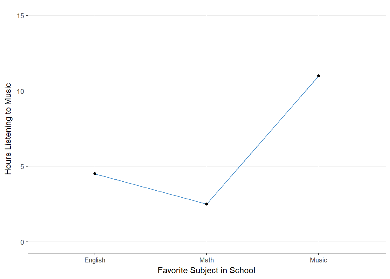
Figure 13.1. Main effect of School.
It seems that those who like the subject of Music tend to listen to more music than those who prefer Math or English
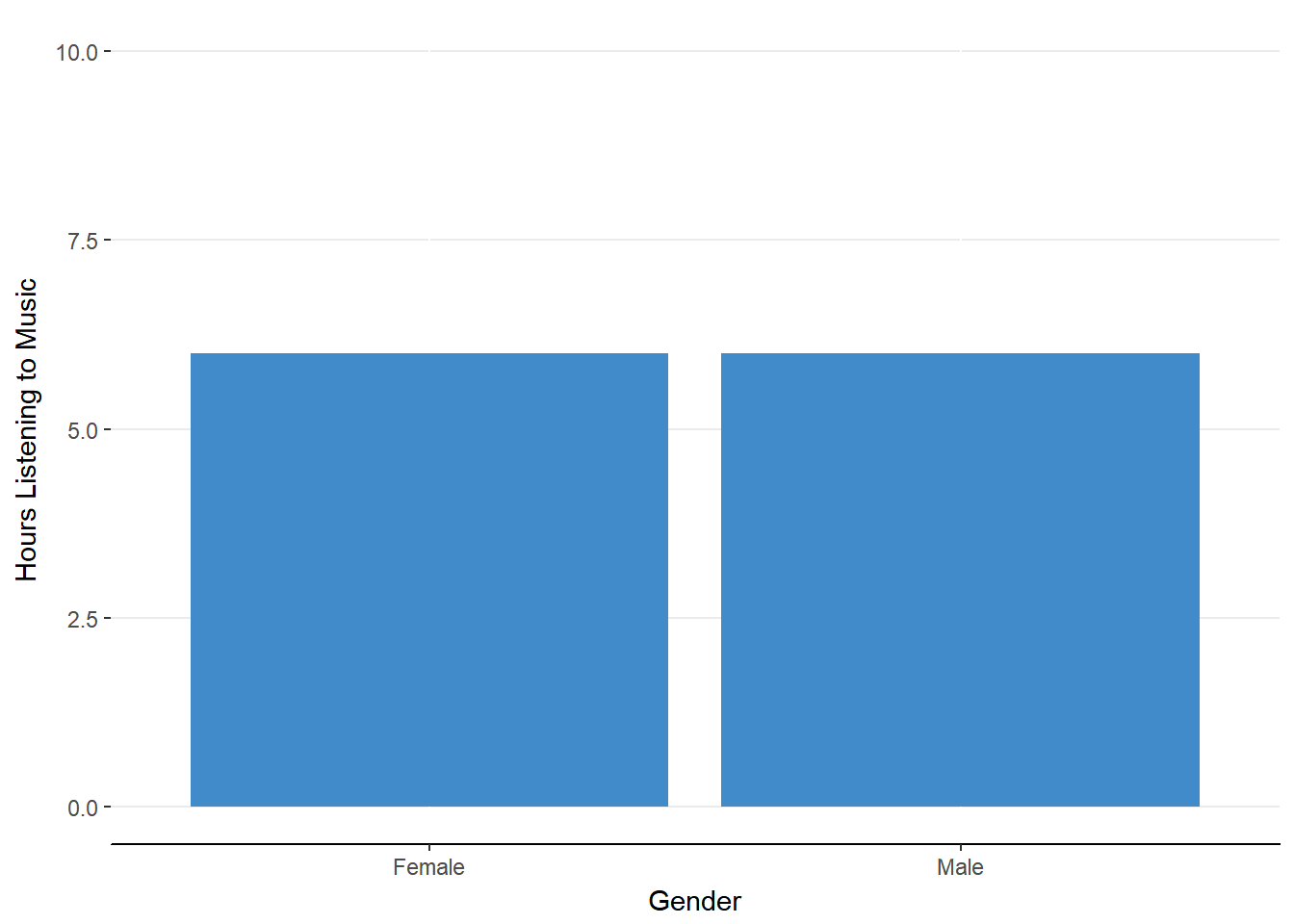
Figure 13.2. Main effect of Gender.
There doesn’t appear to be a difference in listening habits of Males and Females.
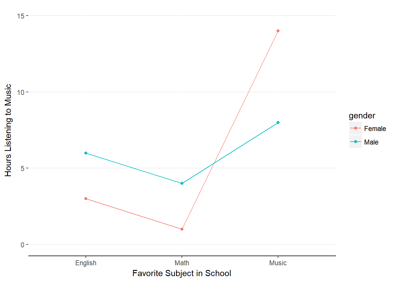
Figure 13.3. Interaction effect of School x Gender
This chart indicates that Females who prefer Music to Math or English listen to music more than the other groups of individuals.
There are two types of interaction plots. A crossover plot indicates a change in the direction of the relationship between one IV and the DV across the levels of the other IV. 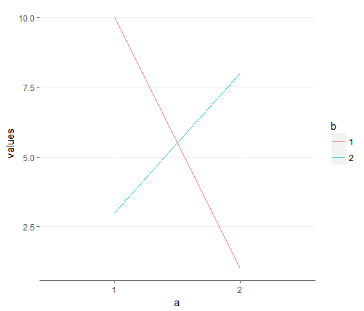 An ordinal plot indicates that the relationship between one IV and the DV is enhanced across the levels of the other IV
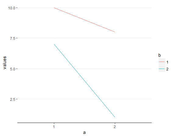
Now we can more fully explored the sources of variance in the expanded ANOVA table.
Between-Groups
This source of variance represents all of the variance due to our independent variables. It includes the variance due to our main effects and interaction effects. It is not necessary to calculate this inclusive source of variance but it allows for a faster approach to finding the interaction sum of squares. Like with the witihin-groups variance, it is easier to subtract some values than to determine the interaction sum of squares directly.
To find the complete between-groups sum of squares, we need to find the difference between each cell mean and the grand mean. To ensure that we include all of the values, we will weight each squared difference according to the number of observations per cell.
In our example, we have 3 observations per cell, a grand mean of 6 and the following cell means: 8, 4, 6, 14, 1, 3. Our equation thus works out as:
\[
\begin{aligned}
\text{SS}_{\text{Between}} &=\Sigma[n(M_{kj}-GM)^2] \\
&= 3(8-6)^2 + 3(4-6)^2 + 3(6-6)^2 + 3(14-6)^2 + 3(1-6)^2 + 3(3-6)^2 \\
&= 3(2^2)+3(-2^2) + 3(0^2)+3(8^2)+3(-5^2)+3(-3^2) \\
&=12 + 12+0+192+75+27 \\
&=318
\end{aligned}
\]
Main Effect: School Subject
This source of variation represents the overall effect of favorite school subject, regardless of one’s gender. We calculate this sum of squares in much the same way as the overall between-groups sum of squares but we will only compare the marginal means for school subject and weight the difference scores according to the number of observations per column.
Our example yielded the following marginal means for Music, Math, and English (respectively): 11, 2.5, and 4.5. Our grand mean is still 6. The equation thus yields:
\[
\begin{aligned}
\text{SS}_{\text{school}} &= \Sigma[nj(M_k - GM)^2] \\
&= 3*2(11-6)^2 + 3*2(2.5-6)^2 + 3*2(4.5-6)^2 \\
&=6(5^2) + 6(-3.5^2) + 6(-1.5^2) \\
&=6*25 + 6*12.25 + 6*2.25 \\
&=150 + 73.5 + 13.5 \\
&=237
\end{aligned}
\]
Main Effect: Gender
We’ll find the overall impact of gender, regardless of school subject in much the same way we had for the impact of school subject. We’ll compare the marginal means for gender to the grand mean and weight each difference by the number of observations per row.
For our example, we have the marginal means for males (Mmales = 6) and females (Mfemale = 6). The grand mean is the same (6). Do you know the sum of squares before we get started? Let’s just confirm the suspicion .
\[
\begin{aligned}
\text{SS}_{\text{gender}} &= \Sigma [nk(M_j - GM)^2] \\
&= 3*3(6-6)^2 + 3*3(6-6)^2\\
&=9*0 + 9*0 \\
&=0 + 0 \\
&=0
\end{aligned}
\]
That’s right. The variance is 0 because each group mean is equal to the grand mean,
Interaction Effect: School x Gender
Now that we’ve found the total variance accounted for by between-groups factors, we can subtract away our main effects to find the variance due to the interaction effect. Remember that the interaction effect represents the change in how one IV impacts the DV because of the levels of the other IV.
\[
\begin{aligned}
\text{SS}_{\text{school x gender}} &= \text{SS}_{\text{Between}} - \text{SS}_{\text{school}} - \text{SS}_{\text{gender}} \\
&= 318 - 237 - 0 \\
&= 81
\end{aligned}
\]
In our example, there is no extra variance due to the interaction of gender and school. That is, the relationship between gender and music listening habits does not change depending on the individual’s favorite subject in school. The other way of expressing this is to say that the relationship between favorite school subject and hours of music listening does not change based on one’s gender.
Error Term: Within-Groups Variation
As with the One-Way Between-Subjects ANOVA, our error term is the within-groups variance. We will find it in the same way as before: subtracting the between-groups sum of squares from the total sum of squares.
\[
\begin{aligned}
\text{SS}_{\text{Total}} &= \Sigma(X-GM)^2 \\
&= (9-6)^2 + (8-6)^2 + (7-6)^2 + (5-6)^2 + (4-6)^2 + (3-6)^2 + (7-6)^2 + (6-6)^2 + (5-6)^2 + (15-6)^2 + (14-6)^2 + (13-6)^2 + (2-6)^2 + (1-6)^2 + (0-6)^2 + (4-6)^2 + (3-6)^2 + (2-6)^2 \\
&=3^2 + 2^2 + 1^2 + -1^2 + -2^2 + -3^2 + 1^2 + 0^2 + -1^2 + 9^2 + 8^2 + 7^2 + -4^2 + -5^2 + -6^2 + -2^2 + -3^2 + -4^2 \\
&=9 + 4 + 1 + 1 + 4 + 9 + 1 + 0 + 1 + 81 + 64 + 49 + 16 + 25 + 36 + 4 + 9 + 16 \\
&= 330 \\\\
\text{SS}_{\text{Within}} &= \text{SS}_{\text{Total}} - \text{SS}_{\text{Between}} \\
&= 330 - 318 \\
&= 12
\end{aligned}
\]
Let’s update our extended ANOVA table with these sums of squares.
Table 13.6
Factorial ANOVA Table with Sums of Squares
| Between-Groups |
330 |
- |
- |
- |
| - School Subject |
237 |
k-1 |
\(\frac{\text{SS}_{\text{school}}}{df_{\text{school}}}\) |
\(\frac{\text{MS}_{\text{school}}}{\text{MS}_{\text{within}}}\) |
| - Gender |
0 |
j-1 |
\(\frac{\text{SS}_{\text{gender}}}{df_{\text{gender}}}\) |
\(\frac{\text{MS}_{\text{gender}}}{\text{MS}_{\text{within}}}\) |
| - School x Gender |
81 |
(k-1)(j-1) |
\(\frac{\text{SS}_{\text{school x gender}}}{df_{\text{school x gender}}}\) |
\(\frac{\text{MS}_{\text{school x gender}}}{\text{MS}_{\text{within}}}\) |
| Within-Groups |
12 |
N-k*j |
\(\frac{\text{SS}_{\text{Error}}}{df_{\text{Error}}}\) |
- |
| Total |
330 |
N-1 |
- |
- |
Degrees of Freedom
Calculating the sums of squares is always the longest part of ANOVA. Now we can determine the degrees of freedom before we solve for our F-values.
dfSchool = k - 1 = 3 - 1 = 2
dfGender = j - 1 = 2 - 1 = 1
dfSchoolxGender = (k - 1)(j-1) = 2 x 1 = 2
dfwithin= N-kj = 18 - 32 = 18 - 6 = 12
Just to check our work, we’ll find the total degrees of freedom
dfTotal = N - 1 = 18 - 17
Let’s add up our calculated df to ensure it is equal to our total df.
2 + 1 + 2 + 12 = 17
With our SS and df verified, we can find our mean squares and then our F-values
Mean Squares
Remember that the Mean Squares are equal to the sum of squares divided by the degrees of freedom for each effect and error term.
MSschool = \(\frac{\text{SS}_{\text{school}}}{df_{\text{school}}}\) = \(\frac{237}{2}\) = 118.5
MSgender = \(\frac{\text{SS}_{\text{gender}}}{df_{\text{gender}}}\) = \(\frac{0}{1}\) = 0
MS~SchoolxGender = \(\frac{\text{SS}_{\text{school}}}{df_{\text{school}}}\) = \(\frac{81}{2}\) = 40.5
MSwithin = \(\frac{\text{SS}_{\text{within}}}{df_{\text{within}}}\) = \(\frac{12}{12}\) = 1
Given that we have a MSwithin = 1, our F-values will be very easy to calculate.
F-values
To determine the F-values, we need to divide the MS for each effect by the MSwithin.
FSchool = \(\frac{\text{MS}_{\text{School}}}{\text{MS}_{\text{within}}}\) = \(\frac{118.5}{1}\) = 118.5
FGender = \(\frac{\text{MS}_{\text{Gender}}}{\text{MS}_{\text{within}}}\) = \(\frac{0}{1}\) = 0
FSchoolXGender = \(\frac{\text{MS}_{\text{School x Gender}}}{\text{MS}_{\text{within}}}\) = \(\frac{40.5}{1}\) = 40.5
Before we check on the statistical significance of our F-values, we should update our ANOVA Table
Table 13.7
Complete Factorial ANOVA Table
| Between-Groups |
330 |
- |
- |
- |
| - School Subject |
237 |
2 |
118.5 |
118.5 |
| - Gender |
0 |
1 |
0 |
0 |
| - School x Gender |
81 |
2 |
40.5 |
40.5 |
| Within-Groups |
12 |
12 |
1 |
- |
| Total |
330 |
17 |
- |
- |
Critical F-values
We only had one Fcrit for the One-Way Between-Subjects ANOVA and to find that value, we consulted the table using the dfbetween and dfwithin. We will follow the same procedure but we will have to find Fcrit for each effect we are testing.
What degrees of freedom shall we use? We will use the same dfwithin for each Fcrit because we are using the same error term for each F-test. We will need to use the df associated with each effect, however, instead of just one dfbetween.
Fcrit for the main effect of school has 2 and 12 degrees of freedom.
Fcrit = 3.885
Fcrit for the main effect of gender has 1 and 12 degrees of freedom.
Fcrit = 4.747
Fcrit for the interaction effect of School x Gender has 2 and 12 degrees of freedom.
Fcrit = 3.885
Decisions regarding H0
Recall that our null hypotheses are that the groups are from the same population such that:
\[
M_1 = M_2 = ... = M_k = \mu_0
\]
In each effect, we are testing the equality of different sets of means. For the main effects, we are testing if the groups defined by each IV are equal. As such, the null hypothesis for the effect of school is:
\[
M_{\text{Music}} = M_{\text{Math}} = M_{\text{English}} = \mu_0
\]
Similarly for gender, the null hypothesis is:
\[
M_{\text{Male}} = M_{\text{Female}} = \mu_0
\]
The null hypothesis for the interaction effect of School x Gender is that all of the cell means are equal. That is, regardless of the combination of factors, the group means will be equal. The complete statement of H0 is:
\[
M_{\text{Music x Male}} = M_{\text{Music x Female}} = M_{\text{Mathx Male}} = M_{\text{Math x Female}} = M_{\text{English x Male}} = M_{\text{English x Female}} = \mu_0
\]
To overturn a null hypothesis, you need a calculated F-value that is larger than the corresponding critical F-value.
Here are the comparisons
Table 13.8
Comparing Fcrit to Fcalc for each Effect
| School |
118.5 |
3.885 |
Yes |
| Gender |
0 |
4.747 |
No |
| School x Gender |
40.5 |
3.885 |
Yes |
It seems that we can reject H0 for the main effect of favorite subject in school and H0 for the interaction effect of school subject and gender on the number of hours listening to music.
Post-Hoc Analyses
With statistically significant F-values for the main effect of School Subject and the interaction of School x Gender, we only know that at least one of the means is statistically significantly different from the others. To determine which means are different, we will need to perform post-hoc analyses.
The order in which we examine the significant effects matters. If there are significant interaction effects, you need to perform the post-hoc analyses for those interactions before inspecting and interpreting the main effects. This may seems strange. How could the order of interpretation have any implication for the results of our tests? The results still stand that there was a statistically significant difference between group means, but those may not tell the more detailed story revealed by the interaction effect. Check out figure 13.6, which demonstrates a crossover interaction.
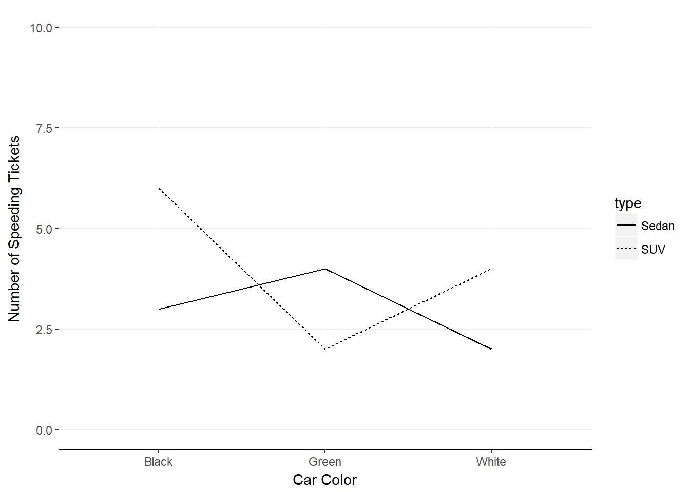
Figure 13.6. Crossover interactions can change the interpretation of main effects.
If we were to assume that there was a main effect of Car Type (ignoring Car Color) on number of speeding tickets, we would not be telling the full truth. That’s because SUVs had more speeding tickets than Sedans only when the cars were Black or White. That is, SUVs had fewer speeding tickets than Sedans when the cars were Green.
The rule is to examine significant interaction effects before examining significant main effects. Effects that did not yield statistically significant F-values do not need further investigation.
Choosing Post-Hoc Comparisons
There can be many means for Factorial ANOVA. We are not required to test each combination of means, however. You should think about the meaningful questions in your design and consult the charts of the data. If you find a significant interaction that involves a variable with more than 2 levels, you may consider performing a Simple Main Effects test.
Simple Main Effects Test
The simple main effects test is a One-Way Between-Subjects ANOVA for just a subset of the data involved in the interaction effect. In our 3x2 example, we found a significant interaction of School x Gender. We could test if there is an effect of school subject for just Males and then if there is an effect of school subject just for Females.
If the F-value is significant for either One-Way ANOVA, you’ll need to perform Tukey HSD to determine which means are statistically significantly different.
If you would rather compare across the other variable (e.g., gender) you can skip right to Pairwise Comparisons using Tukey HSD. Wait! Why not just do the pairwise comparisons and skip the ANOVA? Remember that we need to maintain our family-wise type I error rate. Performing a secondary ANOVA will reduce the likelihood of falsely rejecting a null hypothesis.
Pairwise Comparisons
If you are more interested in how two groups differ within the levels of another variable, you can perform Tukey HSD tests for each comparison.
Our Example
Let’s revisit our interaction plot again.
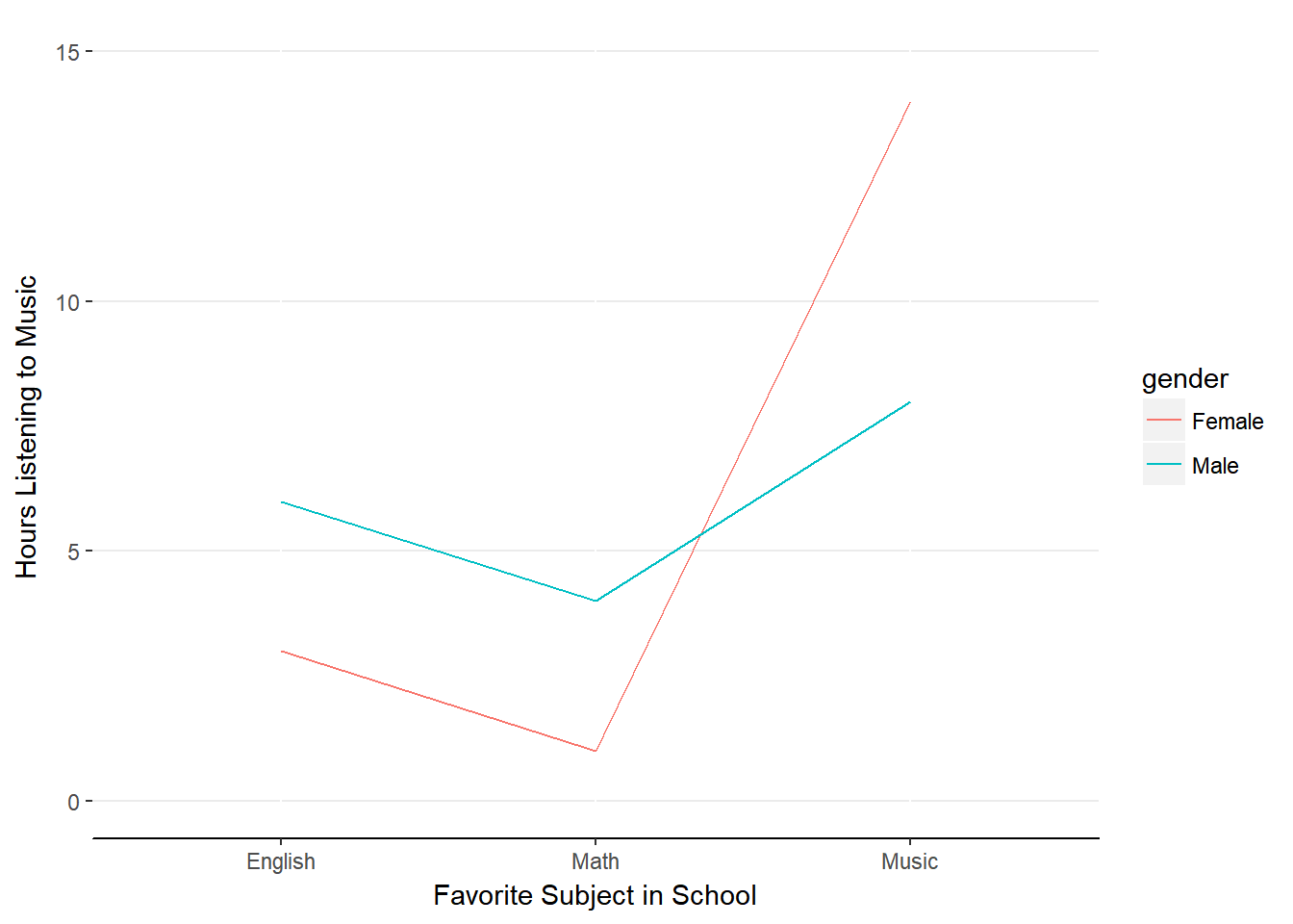
Figure 13.3. Interaction effect of School x Gender
It seems that we have a crossover in the effect of school subject when we get to Music. In our sample, it seems males who preferred Math or English listened to more music than females who preferred Math or English. However, the pattern switches for those who prefer Music: Females tend to listen to more music than males. Because the more interesting pattern involves the gender and the subject of Music, we should investigate the statistical difference between Males and Females who prefer Music and then compare the various marginal means for school subject.
Interaction: Male vs. Female within Music
We’ll need our critical q-value before determining the critical difference. Recall that we need the number of groups and dfwithin to find the critical q-value. For comparisons among cell means for an interaction effect, we will use the number of cell means as the number of groups (k = 6). The within-groups degrees of freedom from the original analysis will also be used (dfwithin = 12). According to the q-table, our critical q-value is 4.750.
To get the critical difference, we need to multiply the critical q-value by the standard error. The full formula is:
\[
q_{\alpha}\sqrt{\frac{MSE}{n}}
\]
where \(q_{\alpha}\) is the critical q-value, MSE is the Mean Square Error (in our case this is the within-groups mean square), and n is the number of observations per group.
Our critical difference is thus:
\[
q_{\alpha}\sqrt{\frac{MSE}{n}} = 4.750 \sqrt{\frac{1}{3}}= 4.750\times0.577 = 2.74
\]
The difference between MusicMales and MusicFemales is 8 - 14 = -6. The difference between is statistically significantly different.
Since we’ve calculated the critical difference for any interaction means, we can also verify if the other means are statistically significantly different.
Table 13.9
Comparison of Mean Difference and Critical Differences for Interaction Means
| MathMale - MathFemale |
3 |
2.74 |
| EnglishMale - EnglishFemale |
3 |
2.74 |
| MusicMale - MusicFemale |
-6 |
2.74 |
This is a helpful table as it shows us that there is a difference among the genders for each School Subject. This is interesting considering that we did not have a main effect of Gender. This is because of the crossover occurring within Music. This is another reason why it is important to investigate interactions before interpreting main effects.
Main Effect: Music vs. Math vs. English
We already know that at least one mean is different across these levels because of our significant main effect for School Subject. We’ll calculate a new critical difference against which we will compare our marginal means. A new critical difference score is needed because we are changing the number of groups and the number of observations per group as we move from cell to marginal means.
We are comparing the three levels of School subject, making k = 3. Our dfwithin is still 12. The new critical q-value is 3.773.
The new critical difference becomes:
\[
q_{\alpha}\sqrt{\frac{MSE}{n}} = 3.773 \sqrt{\frac{1}{6}}= 3.773\times0.408 = 1.54
\]
Let’s construct another comparison table to quickly gauge which marginal means are different.
Table 13.10
Comparison of Mean Difference and Critical Differences for Main Effect Means
| Music - Math |
8.5 |
1.54 |
| Music - English |
6.5 |
1.54 |
| Math - English |
2 |
1.54 |
Once again we find that all of the means are statistically significantly different from the others such that those who prefer Music listen to more music than those who prefer Math and those who prefer Math listen to more music than those who prefer English.
With the ANOVA and post-hoc analyses complete, we are ready to state our conclusion.
Conclusions: Interpreting the results
Here is a review of the results: 1. Significant effect of School Subject 2. Significant interaction effect of School x Gender 3. All cell means different 4. Crossover of pattern for Males and Females who like Math 5. More music listened to by those who like Music > those who like Math > those who English
Our last task is to integrate this information into a cohesive statement.
A 3x2 factorial ANOVA revealed a main effect of School Subject and an interaction effect of School x Gender on the amount of music listened to by high school students. Post-hoc analyses revealed that Males listen to more music than Females across all Subjects, except for when individuals preferred Music. Females who prefer Music listened to more music than Males who prefer Music. Tukey HSD also revealed that individuals who preferred Music listened to more music than those who preferred Math, who also listened to more music than those who preferred English.
Summing Up Two-Way Between-Subjects ANOVA
The two-way between-subjects ANOVA is a generalization of the one-way ANOVA. With this technique, we are able to simultaneously test the impact of multiple categorical variables on a continuous dependent variable. We refer to ANOVA that have more than one IV as Factorial ANOVA. The number of independent variables and the levels of each are indicated in the AxBxC format. For example, a 3x4x2 Factorial ANOVA has 3 IV with 3, 4 and 2 levels for the IVs respectively.
The big advantage is that we can control for Type I error rate while testing differences among many means. We also have the ability divide the variance into main effects and interaction effects. Main effects represent the impact of on IV on the DV, ignoring the other IVS. Interaction effects represent the impact of multiple IVs together on the DV.
Significant effects will require post-hoc analyses to clarify which means are statistically different, providing the number of means to be compared are greater than 2.