By completing this section, you will be able to:
Describe the concept of central tendency
Describe the concept of variability
Define three measures of central tendency
Identify different distribution shapes
Calculate each measure of central tendency
Choose the appropriate measure of central tendency
Define three measures of variability
Calculate each measure of variability
Match measures of central tendency and variability
Professor Weaver’s Take
If you were like me growing up, you spent a lot of your time thinking about what was normal. Of course, by that I mean I was particularly worried that I was not normal. To be normal was to be like everyone else and that seemed to be a good thing. Perhaps that concern for thinking about the totality of everyone else’s behavior informed my desire to be a psychologist and to pursue Statistics. You may not have yet gone as far as I have but I’m sure that desire for knowing where you stand relative to others is nearly universal.
As a grown up, I know that I am not like everyone else and that seems to be a good thing. I have a new appreciation for diversity and variability. As a statistician, I’ve learned that it is easier to decide if a distribution is normal than if I am normal (I’m sure I’m not). As you’ll discover in this module, statistician care a lot about distributions and their properties because this is the basis of our ability to make decisions regarding probability and statistical hypotheses. We’ll cover all of that throughout the rest of the modules. This module will focus how we describe distributions by the relationships among two properties: central tendency and variability.
Describing Distributions
A distribution is a way to organize a set of data for a variable (see the last module). For example, we could rank order the number of text messages each of 50 students sends in one day. We can represent this information in a frequency table (see table 6.1) or a histogram (see figure 6.1).
Table 6.1
Frequency Distribution of Text Messages Sent
| Bin | Count |
|---|---|
| 55-59 | 1 |
| 60-64 | 4 |
| 65-69 | 4 |
| 70-74 | 12 |
| 75-79 | 15 |
| 80-84 | 11 |
| 85-89 | 2 |
| 90-95 | 1 |
| Total | 50 |
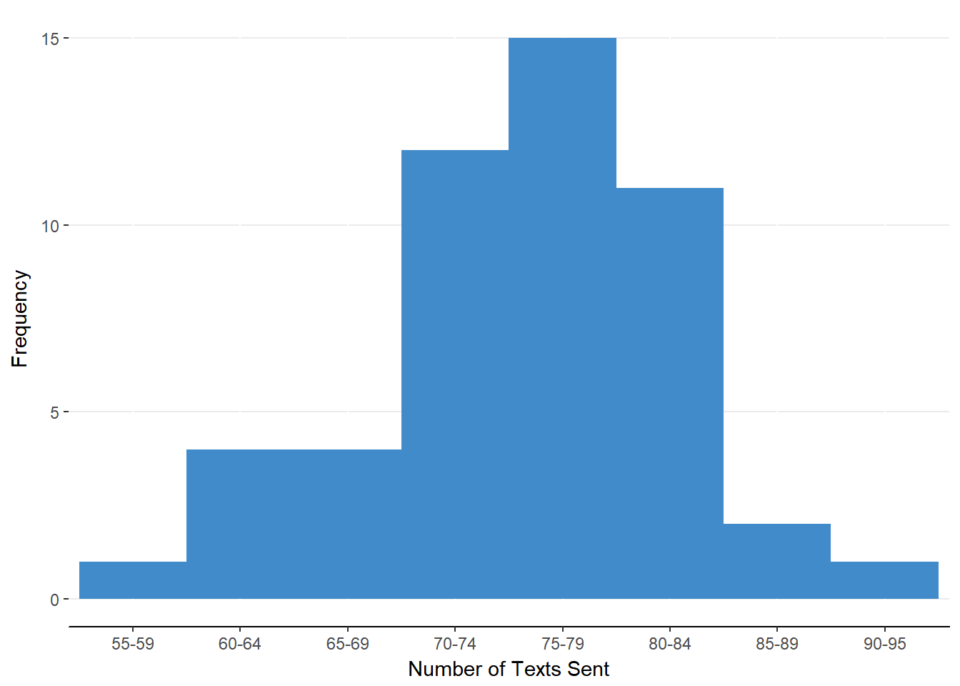
Figure 6.1. Histogram of number of text messages sent for each of 50 students in one day.
One of the users of Statistics is to summarize and classify to make more clear patterns. Just as we’ve done for data and variables before, we can do for distributions. We will find that assigning a category for a distribution will help guide or decisions about the tires of analyses that are appropriate for our data. There are many times of distributions but we will restrict our scope to normal and skewed.
A normal distribution is bell-shaped and symmetrical around the peak (see figure 6.2). A skewed distribution is asymmetrical about the peak (see figure 6.3). To mathematically define the normality of a distribution, we must first define two important features of any distribution: central tendency and variability.
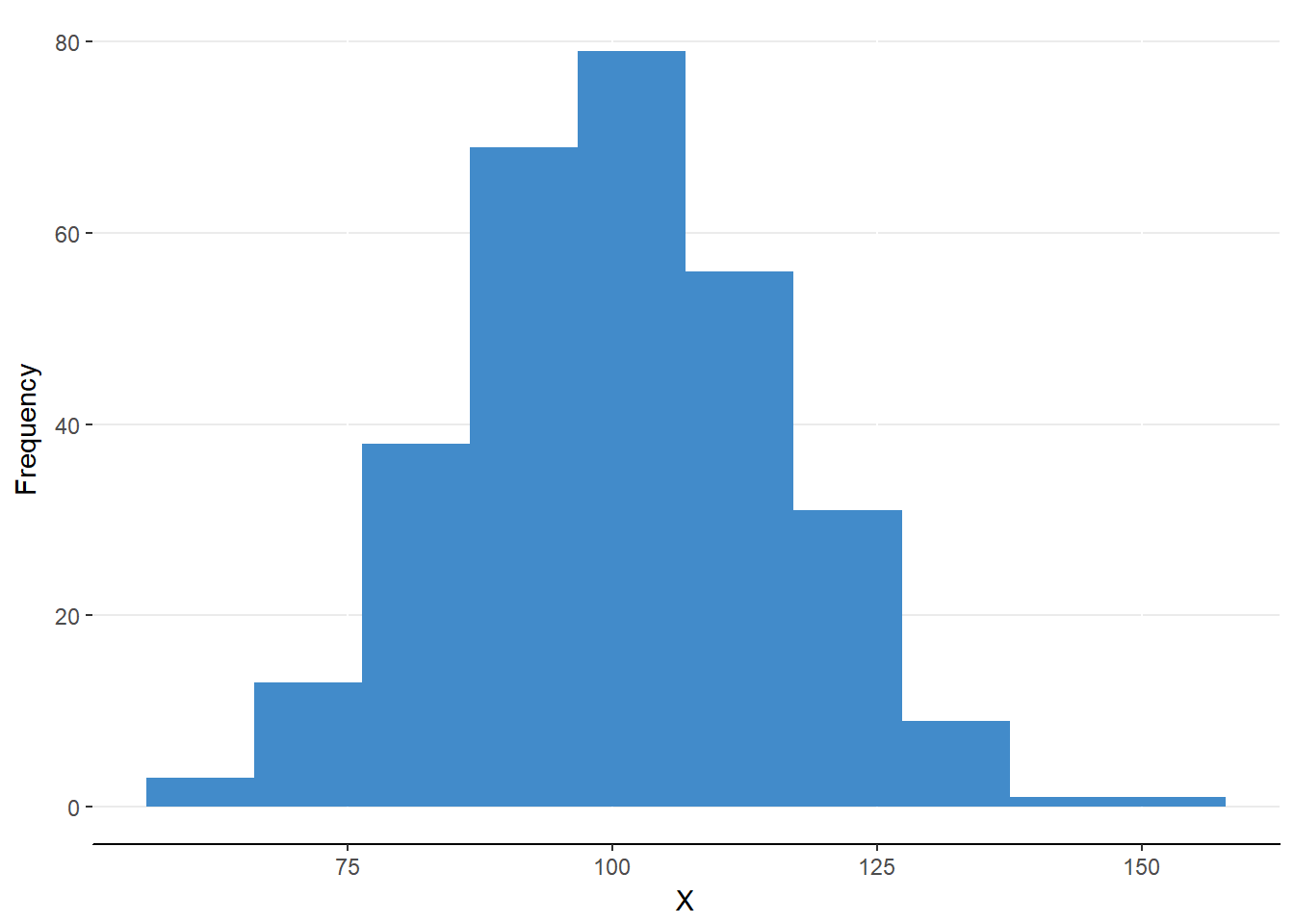
Figure 6.2. A normal distribution
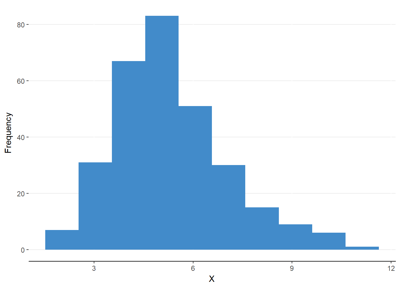
Figure 6.3. A skewed distribution
Measures of Central Tendency
Central tendency refers to the measures of the value or values that represents the center of a distribution.
Defining centrality can be a bit difficult because there are various aspects of centrality that we can consider. To better understand this difficulty, let us think about a city rather than a distribution of data. We might consider the center of the city to be where most of the people live. Rather than residence, we could focus on where most of the people like to spend their money; the commercial center. Lastly, perhaps we may define the center geographically. Each of these would provide some different information about the city.
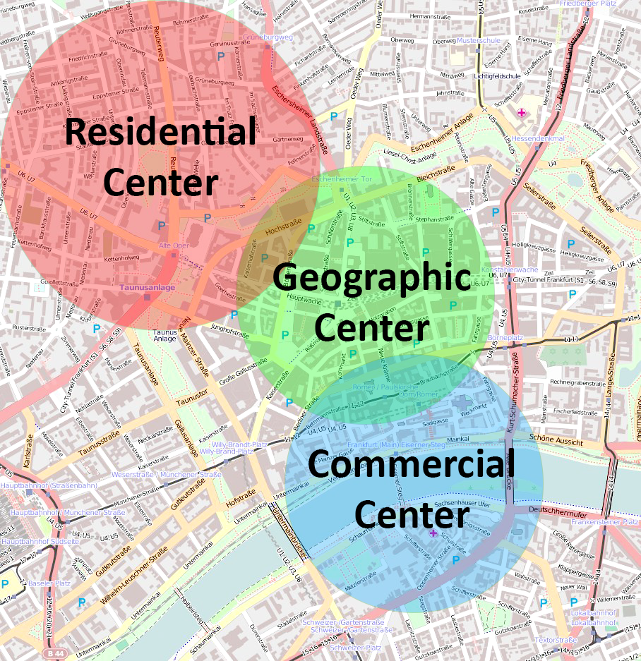
Figure 6.4. Various city centers. Altered from original image (Wikimedia, 2011).
Similarly, we can describe the center of a distribution is several ways to gain different information about the distribution.
Mode
The mode is the most frequently occurring value in the distribution. This value will correspond with the peak of the histogram for the distribution. You can also scan through a frequency distribution to find the value that corresponds to the largest frequency or count.
The mode is the most frequently occurring value
For some distributions, there can be more than one pronounced peak in the distribution. We call these multimodal distributions. Check out figure 6.5 and try to determine why there are two modes.
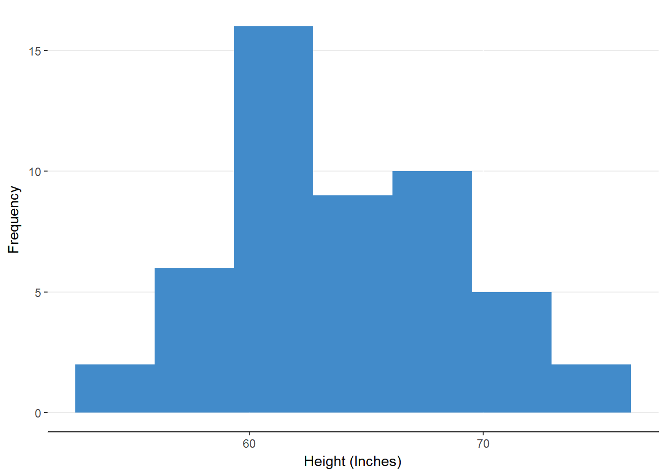
Figure 6.5. A multimodal distribution
These multiple peaks are usually a result of having two distributions combined into one. In the case of figure 6.5, there are two modes for height because the distribution of heights for women and for men have been combined. Thus, there is a mode for women and a mode for men. We’ll discuss how statistical models can represent the impact of various predictor variables (e.g., sex) and a dependent variable (e.g., height) in future modules.
Although the mode can nicely correspond with the center of a distribution and is very easy to determine, it does not utilize very much information from the distribution. Rather than telling us about the various values in the distribution, it only tells us about one value. There is a silver lining here. The mode only requires us to count values, which means that we can indicate the mean of any variable. We can represent the mode of popular dog names (nominal scale), of stress ratings during final exams week (ordinal scale), of bank account balances (interval scale), and of the number of minutes of exercise a student gets each day (ratio scale).
Median
The median is often a more useful measure of central tendency when working with ordinal, interval, or ratio data because it Incorporated the ranking of the values rather than just the count or frequency of the values. As you may recall from earlier modules, the median is the value at which 50% of values are below and 50% of values are above. That is, if we order the values from smallest to largest and count halfway through the values, the median will be at the dividing point.
The median is the value at half-way point in ordered data
The location of the median is at \(\frac{n + 1}{2}\) where n is the number of values. If the median is at the halfway point, you may be wondering why the median is not at \(\frac{n}{2}\). Let’s find the median of the following 10 ordered values (number of yawns per student during a 30 minute lecture) to find out.
2 3 5 5 6 8 10 11 13 15
According to our formula, the median is at \[\frac{n+1}{2} = \frac{10 + 1}{2} = \frac{11}{2} = 5.5.\]
Of course, there isn’t a value at 5.5 so we will have to go halfway between the value at location 5 and location 6. To do that, we add the two values and divide by 2.
\[ \frac{\text{Location Below} + \text{Location Above}}{2} = \frac{6 + 8}{2} = \frac{14}{2} = 7 \]
Let’s rewrite our ordered values and insert the median
2 3 5 5 6 7 8 10 11 13 15
Notice how there are five values below the median and five values above the median. Because we have 10 values, 5/10 = .50 = 50% above and below the median. If we would have used \(\frac{n}{2}\), we would have chosen the value at 5 (which is 6), leaving 4 values (40%) below the median and 5 values (50%) above the median. By definition, using \(\frac{n}{2}\) will not yield the median.
Finding the mean of an odd number of ordered values is even easier because there is a value that divides the data into two equal parts. Let’s add another value to our list to see this.
2 3 5 5 6 8 10 11 13 15 29
Our list now has 11 values so or median is located at \(\frac{11 + 1}{2} = \frac{12}{2} = 6\). Counting from the left six values we find 8.
2 3 5 5 6 8 10 11 13 15 29
Once again, the data are divided in half with 5 values below and five values above the median.
Let us compare the median and mode of our data. The mode is five and the median is 8. Which value best represents the center of the data? Which value is more informative? Because the media incorporates the relative position of the values, we would use this value as a better representation of central tendency than the mode. However, this does not mean that the mode is not informative. It still tells us which value occurred most often. Soon, we will compare all our values of central tendency to help us determine how skewed or normal a distribution is.
The median utilizes information (i.e., order) of values but leaves out the values themselves. The last measure of central tendency incorporates the values of each datum in finding the balancing point in the data.
Mean
Reviewing quickly, the median is the value at the 50% mark or 50th percentile and the mode is the most frequently occurring value. The mean is the value at which the values below the mean balance out the values above the mean. It is calculated by taking the arithmetic mean or average of all the values.
Let us work with our current set of values:
2 3 5 5 6 8 10 11 13 15 29
The mean is calculated as
\[ \overline{x} = M=\frac{\sum_{i = 1}^{n}x_{i}}{n} = \frac{x_{1} + x_{2} + \ldots + x_{n}}{n} =\frac{2 + 3 + 5 + 5 + 6 + 8 + 10 + 11 + 13 + 15 + 29}{11}=\frac{107}{11}=9.73 \]
A few notes on the symbols you see. \(\overline{x}\) is pronounced “x bar” and is often used to represent the sample mean. Other times a capital “M” is used to represent a sample mean. ?? is the Greek letter “sigma.” This symbol is used to indicate that you will be adding together a series of numbers to the right of the symbol. In the extended form shown above, there is a starting location value and an ending value for the data. The starting value is below sigma (i = 1) that tells us to start with the first value. The ending value is above sigma (n is a representation of sample size) that tells us to add all the values until we reach the last value. Each value in the dataset can be represented as xi where i is the location of the value in our series of numbers. Table 6.2 shows the correspondence between xi values and the numbers in our series.
Table 6.2
Matching data values to xi representation
| Xi | Value |
|---|---|
| X1 | 2 |
| X2 | 3 |
| X3 | 5 |
| X4 | 5 |
| X5 | 6 |
| X6 | 8 |
| X7 | 10 |
| X8 | 11 |
| X9 | 13 |
| X10 | 15 |
| X11 | 29 |
We will have more practice with this sigma notation shortly when we discuss standard deviation. In short, just remember that sigma notation tells you what to add up.
Now let us get back to the mean. Recall that we can conceptualize the mean as a balancing point for our data. Let’s build out this balancing metaphor by imagining that each value is connected to the mean with a metal rod such that the length of the rod is the numerical distance between the value and the mean. We’ll pair up values so that the most extreme (2 and 29) are connected to the mean followed by the next extreme (3 and 15) and so forth. Because we have an odd number, one score (10) will not have a counter balancing point.
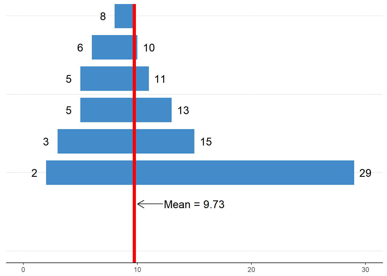
Figure 6.5. Visualizing the mean as a balancing point
Although we may have fewer values on the right side of the scale, there is a much longer bar that compensates for the fewer and shorter bars compared to the left side. As such, the mean is the point at which the sum of the distances between the values and the mean balances out (i.e., equal to zero).
Rather than the graphic representation of distances, let us calculate the actual distance between the values and the mean.
Table 6.3
Balancing distances above and below the mean.
| Xi | Xi - M | |
|---|---|---|
| 2 | 2-9.73 = -7.73 | Distances below the mean add to -29.38 |
| 3 | 3-9.73 = -6.73 | |
| 5 | 5-9.73 = -4.73 | |
| 5 | 5-9.73 = -4.73 | |
| 6 | 6-9.73 = -3.73 | |
| 8 | 8-9.73 = -1.73 | |
| 10 | 10-9.73 = 0.27 | Distances above the mean add to 29.35 |
| 11 | 11-9.73 = 1.27 | |
| 13 | 13-9.73 = 3.27 | |
| 15 | 15-9.73 = 5.27 | |
| 29 | 29-9.73 = 19.27 | |
| \(\sum_{}^{}{(x_{i} - M)} = -0.03\) |
The sum of the distances between the values below the mean and the distances between values above the mean cancel each other out (the -0.03 is due to rounding error). We can now be sure that our calculated mean is indeed the balancing point for our data.
The mean is a very informative measure of central tendency because it incorporates the value of each datum in the calculation. There are restrictions as to the data for which we can calculate the mean. We can only calculate the mean for data that have equal spacing between values on the scale on which it is measured. That is, we can only calculate the mean for interval and ratio scales of measurement.
Let us review the three measures of central tendency discussed thus far.
Table 6.4
Comparison of three measures of central tendency
| Measure of Central Tendency | Definition | Determination | Scale of Measurement Requirement |
|---|---|---|---|
| Mode | Most frequently occurring value | Find value that appears most in data set (e.g., at peak of histogram or bar chart) | Nominal, Ordinal, Interval, Ratio |
| Median | Value at which 50% of data are above / below | Order values from smallest to largest, find value at \(\frac{n + 1}{2}\) | Ordinal, Interval, Ratio |
| Mean | Balancing point for data | Calculate average by adding up all values and dividing by the number of values (n) \[ \frac{\Sigma{X_i}}{n}\] | Interval, Ratio |
Central Tendency and Normality
The three measures of central tendency can be compared for any set of data measured on interval or ratio scales to determine if the distribution is skewed from normality. Remember, a distribution is considered skewed when it is not symmetrical about the peak. This can happen when there is an extreme value above or below the central tendency that is not matched by an extreme value on the other side. When the values are balanced, the mean equals the median, which equals the mode. This occurs in a normal distribution (see figure 6.6).
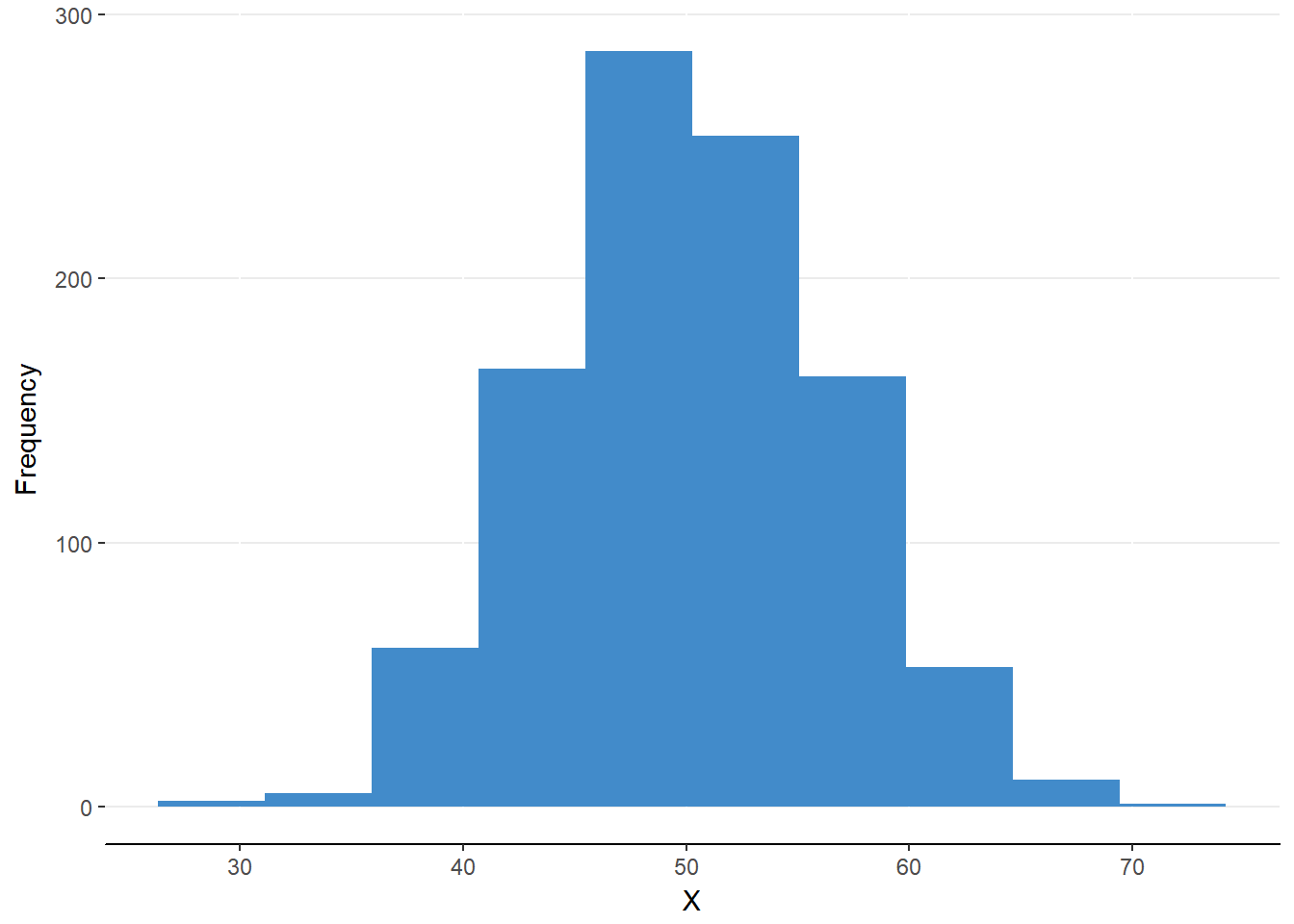
Figure 6.6. A normal distribution
Look at the distribution in figure 6.7. You will notice that the distribution seems to be stretched to the right. The three measures of central tendency have been marked on the distribution as well. The mode is at the peak, the median is just to the right of the mode, and the mean is even further to the right. When the mean is greater than the median and the mode, the distribution is classified as “positively skewed” or “right skewed”. The reason for this positive skew toward the right of the number line is because of the unbalance of extreme values to the right or positive side of the mean.
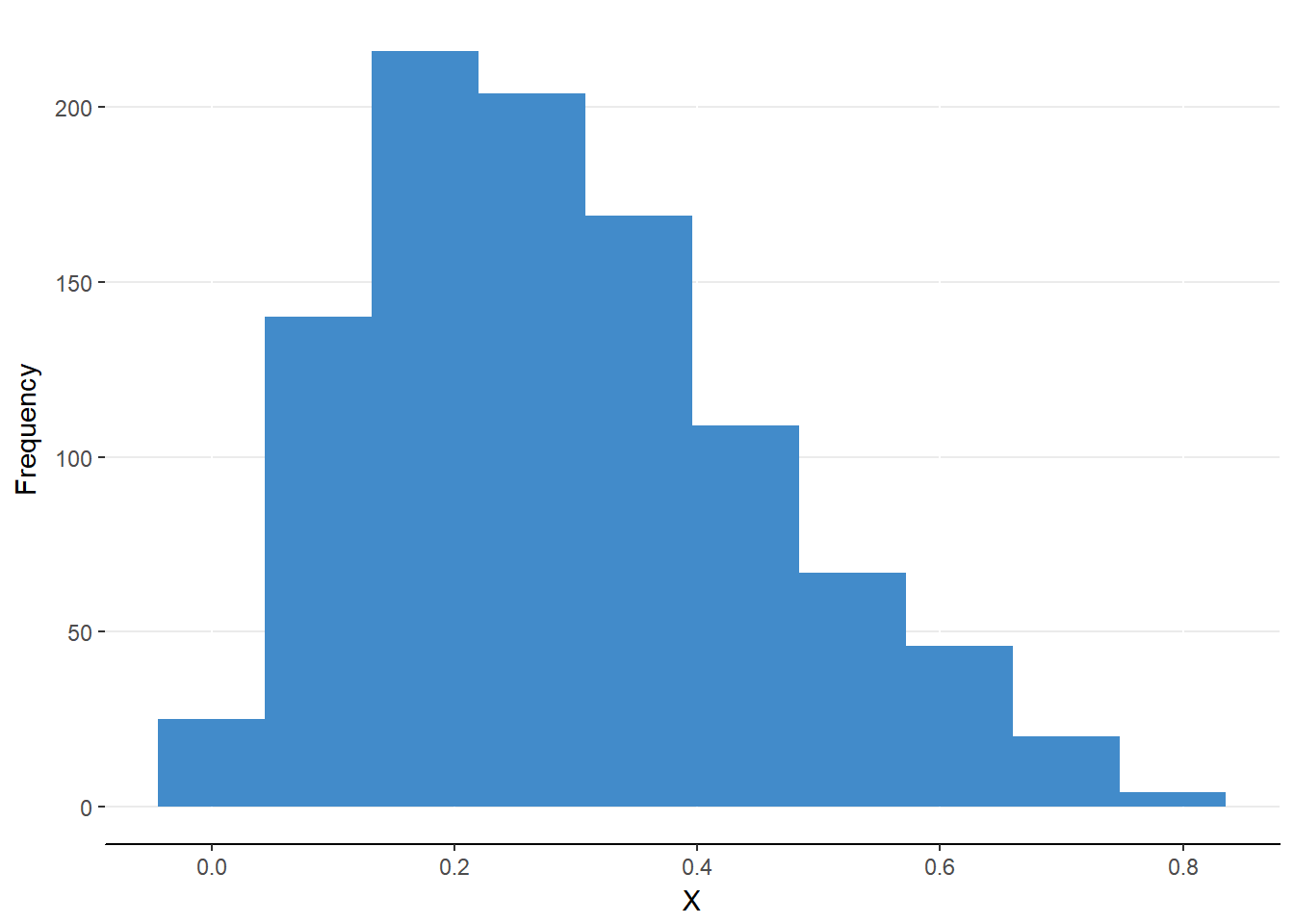 Figure 6.7. A positively skewed distribution
Figure 6.8 shows the opposite scenario; a “left skewed” or “negatively skewed” distribution. In these cases, the mean is less than the median and the mode because the unbalanced extreme value is to the left of the mean.
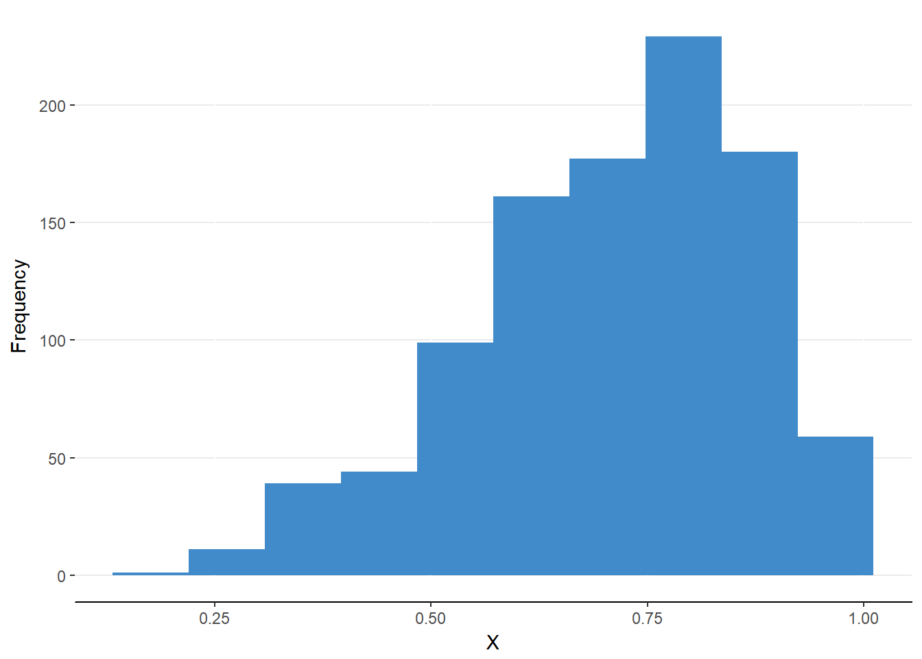
Figure 6.8. A negatively skewed distribution
These skewed distributions help to illustrate that the mean is influenced by these extreme, unbalanced values. As such, the mean no longer seems to represent the center of the distribution. When the distribution is skewed, it is best to use the median because it is not influenced by the extreme values and only deviates slightly from the center. It is still preferable to the mode because it utilizes the rank information of the data.
Although there are many statistical procedures that are based on the rank of data and thus the median, this course will focus mostly on “parametric statistics.” Parametric statistics are those that use the mean and associated measures to make estimates about populations based on samples. To use the mean, we will need normal distributions.
Where We Are Going
We’ve just learned the ways in which we can summarize the middle of a data set or distribution and we’ve discussed when to use the various measures of central tendency. We must go further than just describing the center of a distribution. We need to express that there are different scores within a dataset in a summative form. Click the “Next” button below to learn about measures of variability.