Variability
Take a look at the next two distributions. How are they similar? How are they different?
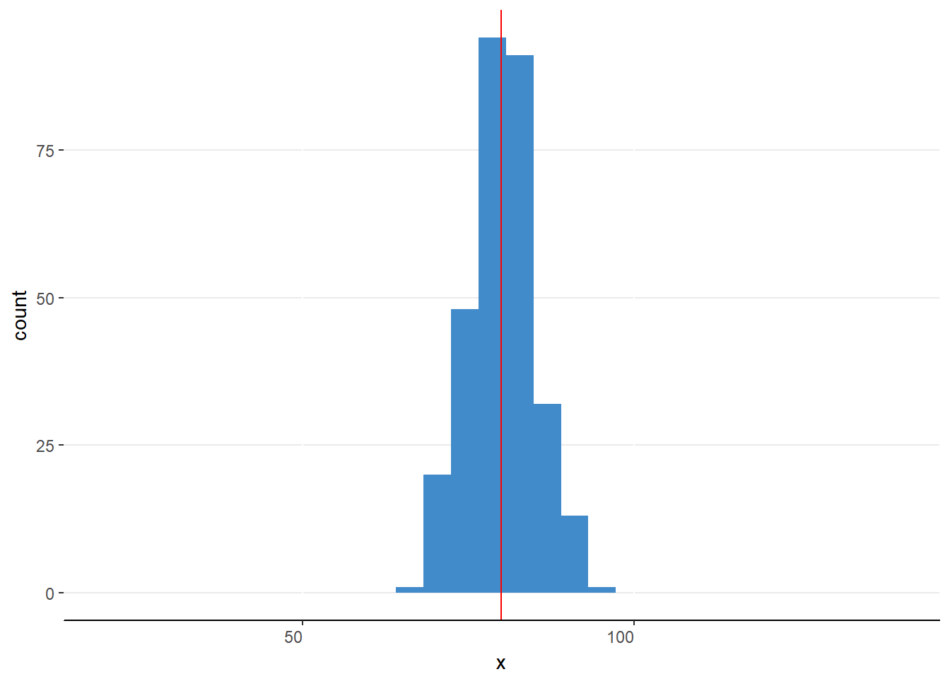
Figure 6.9. A narrow distribution with mean equal to 80.
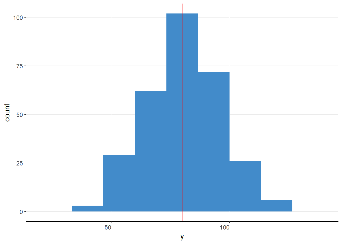
Figure 6.10. A wide distribution with mean equal to 80.
The distributions in figures 6.9 and 6.10 are clearly different distributions yet they have the same measures of central tendency. That is, although the means, medians, and modes are equal in these distributions, something else is different.
Think about this scenario. An economics researcher finds the median income of two cities to be $75,000. Interestingly, one city is the home of 6 well known multimillionaires whereas the other city has no one that reports an income above $150,000. The difference lies not with the center of the income distributions but rather with the extremes of the distribution.
It is not enough to describe a distribution by the central tendency; one also needs to describe how alike or different the values are within the distribution. We have several measures of the variability of a distribution to help better describe the data.
Measures of Variability
Range
The range is the distance between the largest and the smallest value in the data. In our yawning students example, the maximum number of yawns is 15 and the minimum is 2. The range is thus 15 – 2 = 13 yawns. Reporting the range can help summarize how far apart any two values can be. For example, knowing that one lecture recorded a range of 100 yawns whereas another recorded a range of yawns can tell you something about how differently students react to each instructor. Although this is useful, it is a limited measure. It only uses two values and it doesn’t describe how most of the data are spread out in the distribution.
The range is equal to the maximum minus the minimum.
Interquartile Range
The interquartile range or IQR is still a range, but it is more directed than the general range. It describes how far apart the center 50% of data are. It requires that we divide our distribution into four sections or quartiles. These quartiles mark the 25%, 50%, 75% and 100% points of the data. Let us walk through this process before finding the IQR.
The interquartile range or IQR is the range that spans the middle 50% of the data.
Finding Quartiles
We previously found the median (50th percentile) for these data between the 5th and 6th value. The value we calculated was 7.
| X | 2 | 3 | 5 | 5 | 6 | 7 | 8 | 10 | 11 | 13 | 15 |
|---|---|---|---|---|---|---|---|---|---|---|---|
| Quartile | 2nd |
We now need to divide the lower half of the data in half again. Because we have an odd number (nlower = 5), we can simple circle the middle number. The 1st quartile (25th percentile) is 5. Repeat the procedure for the upper half of the data to find the 3rd quartile (75th percentile) at 11. The 4th quartile is the 100^th percentile or the maximum (15).
| x | 2 | 3 | 5 | 5 | 6 | 7 | 8 | 10 | 11 | 13 | 15 |
|---|---|---|---|---|---|---|---|---|---|---|---|
| Quartile | 1st | 2nd | 3rd | 4th |
We have thus found the following values for our quartiles
Table 6.5
Quartiles for Yawns during Lecture
| Quartile | Value |
|---|---|
| 1st | 5 |
| 2nd | 7 |
| 3rd | 11 |
| 4th | 15 |
Calculating the IQR is straightforward. Simply subtract the 1st quartile from the 3rd quartile.
\[ IQR = Q_{3} - Q_{1} = 11 - 5 = 60 \]
This tells us that the center 50% of the data are spread across 6 yawns. Since we located all of the quartiles, let us explore the remaining values. Twenty five percent of students in our sample yawned fewer than 7 times (Q1) and that 25% of students yawned more than 11 times (Q3).
Just like the range, a larger IQR suggests greater variability than a smaller IQR. Let us compare two distributions. Both have maximums of 15 yawns and the minimums of 2 yawns but the first has an IQR of 11 whereas the other has an IQR of 3. The second distribution with an IQR of 3 suggests that the central 50% of students had very similar counts of yawns. The first distribution with an IQR of 11 suggests that the central 50% of students had very different yawn counts.
The IQR is more informative than the range but it still does not use all the available information. It does not tell you how all the data are spread out.
Variance
Whereas the other measures of variability may have had a thread of familiarity, variance tends to be a completely foreign concept for those who are uninitiated to statistics. Variance (s2) is the average of the squared differences between each value and the sample mean. It is a valuable measure of variability of data because it provides one number that indicates how spread out each value is, on average, from the center of the distribution. Before we calculate variance for our example data, let us appreciate the limitations for this measure.
Variance (s2) is the average squared distance of each value and the mean.
First, because we are comparing each value to the mean, we must have a normal distribution without extreme, unbalanced values. Second, because we will be squaring each of the differences between values and the mean, the interpretation of the units can be confusing. In our example, we will be reporting variance in terms of yawns2. I don’t know about you, but I’m not sure how one can square a yawn. Luckily for us, we can simply take the square root to get standard deviation (s) and units that are easier to interpret.
Standard Deviation (s) is the square root of variance.
If squares add such a problem with interpretation, why should they be squared at all? Recall our definition of the mean: it is the balancing point in our data. That is, the values below the mean cancel out the values above the mean. If we are comparing each value to the mean and then adding them up, we will end up with a variance of 0 for every distribution. A constant does not seem like a good option for describing how distributions differ in their spread. To overcome this, we ensure that all of the differences are positive by squaring the differences.
Calculating Variance
The formula for variance can be a little daunting but once you learn how to turn equations into a set of steps, it is as easy as filling in a table.
\[ s^{2} = \frac{\sum_{i = 1}^{n}\left( x_{i} - M \right)^{2}}{n - 1} \]
Just as a reminder, xi is the current value in our data (counting from the first, i=1, to the last, i=n) and M is the sample mean. Sigma (Σ) indicates that we will be adding up what is to the right. In our case, that will be the square of each value minus the mean.
Let us break down this equation into easy to follow steps by following arithmetic order of operations (remember PEMDAS).
Step 1: Parentheses – Subtract the mean from each value
Note, if you haven’t yet calculated the mean, you can do this by adding up the values and dividing by the number of values
Take each value in the dataset and subtract from it the mean. Simply repeat this as you go down your table.
| Xi | Xi - M |
|---|---|
| 2 | 2 – 7.8 = -5.8 |
| 3 | 3 – 7.8 = -4.8 |
| 5 | 5 – 7.8 = -2.8 |
| 5 | 5 – 7.8 = -2.8 |
| 6 | 6 – 7.8 = -1.8 |
| 8 | 8 – 7.8 = 0.2 |
| 10 | 10 – 7.8 = 2.2 |
| 11 | 11 – 7.8 = 3.2 |
| 13 | 13 – 7.8 = 5.2 |
| 15 | 15 – 7.8 = 7.2 |
| \(M=\Sigma{x_i}/n=78/10=7.8\) | \(\Sigma{(x_i-M)}=0\) |
Step 2: Exponents – Square each difference score
Add another column to your table for your squared values. To ensure that we account for all of the differences when we add them up, we need to square each difference value.
| Xi | Xi - M | (xi – M)2 |
|---|---|---|
| 2 | 2 – 7.8 = -5.8 | -5.82 = 33.64 |
| 3 | 3 – 7.8 = -4.8 | -4.82 = 23.04 |
| 5 | 5 – 7.8 = -2.8 | -2.82 = 7.84 |
| 5 | 5 – 7.8 = -2.8 | -2.82 = 7.84 |
| 6 | 6 – 7.8 = -1.8 | -1.82 = 3.24 |
| 8 | 8 – 7.8 = 0.2 | 0.22 = 0.04 |
| 10 | 10 – 7.8 = 2.2 | 2.22 = 4.84 |
| 11 | 11 – 7.8 = 3.2 | 3.22 = 10.24 |
| 13 | 13 – 7.8 = 5.2 | 5.22 = 27.04 |
| 15 | 15 – 7.8 = 7.2 | 7.22 = 51.84 |
| \(M=\Sigma{x_i}/n=78/10=7.8\) | \(\Sigma{(x_i-M)}=0\) |
Step 3: Summation – Add up all the squared differences
At the bottom of the table, add up the squared difference scores. This will give you the “sums of squares” or “SS”. We’ll be calculating a lot of sums of squares for our tests of significance later in the course. I have no doubt that you will become a master of SS in a few weeks time.
| Xi | Xi - M | (xi – M)2 |
|---|---|---|
| 2 | 2 – 7.8 = -5.8 | -5.82 = 33.64 |
| 3 | 3 – 7.8 = -4.8 | -4.82 = 23.04 |
| 5 | 5 – 7.8 = -2.8 | -2.82 = 7.84 |
| 5 | 5 – 7.8 = -2.8 | -2.82 = 7.84 |
| 6 | 6 – 7.8 = -1.8 | -1.82 = 3.24 |
| 8 | 8 – 7.8 = 0.2 | 0.22 = 0.04 |
| 10 | 10 – 7.8 = 2.2 | 2.22 = 4.84 |
| 11 | 11 – 7.8 = 3.2 | 3.22 = 10.24 |
| 13 | 13 – 7.8 = 5.2 | 5.22 = 27.04 |
| 15 | 15 – 7.8 = 7.2 | 7.22 = 51.84 |
| \(M=\Sigma{x_i}/n=78/10=7.8\) | \(\Sigma{(x_i-M)}=0\) | \(\Sigma{(x_i-M)^2}=169.6\) |
Step 4: Division – Divide the Sum of Squared Differences by n-1
Recall that variance summarizes how different each score is from the mean, on average. Just like the mean, we’ll need to divide out the sum by the number of observations. There is a little hitch, we’ll be dividing by n-1 rather than n. This will keep us from a biased estimate of the population variance (more on that soon).
\[ s^{2} = \frac{169.6}{10 - 1} = \frac{169.6}{9} = 18.84 \]
Just like or other measures of variability, the larger the number, the more variability. There are some properties of variance that are worth noting. The minimum variance for any distribution is zero. A distribution that has only one value would have a variance of zero. There is no upper limit for variance, meaning that the only constraint are the possible values in the data. Lastly and most importantly, because variance used all the data, it can be influenced by this extreme, unbalanced values. Just as we discussed with the mean, it is best to use the variance only when the distribution is approximately normal. These properties are also true for standard deviation.
Calculate Standard Deviation
The simple transformation from variance to standard deviation is taking the square root of variance. The advantage is offering a summary of variability in the same units as the data.
\[ s = \sqrt{18.84} = 4.34 \]
In our example the data vary by 4.34 yawns from the mean, on average. Apart from the ease of interpretation, we’ll later find that we can transform or values into standard deviation values that will allow us to compare relative positions of values across different distributions. For now, just appreciate that standard deviation is a useful measure of variability that will have many implications for how we make decisions in parametric statistics.
The Five-Number Summary
The best ways to describe a distribution is to provide multiple descriptive statistics. One of my favorites is the five-number summary, so-called because it includes five of the descriptive we’ve covered: Minimum, Median, Mean, Standard Deviation, and Maximum. By presenting these values, one is able to judge the range, the variability, central tendency, and an approximation of skew by comparing the mean and mode.
Table 6.6
Five Number Summary
| Statistic | Minimum | Median | Mean | SD | Maximum |
|---|---|---|---|---|---|
| Value | 2 | 7 | 7.8 | 4.30 | 15 |
A similar set of numbers is often graphed. A box-and-whiskers plot (shown in figure 6.11) marks the minimum with a line (the lower whisker), the first quartile with the bottom of the box, the median with a line inside the box, the third quartile with the top of the box, and the maximum with the upper whisker. These graphs are great for comparing multiple distributions.
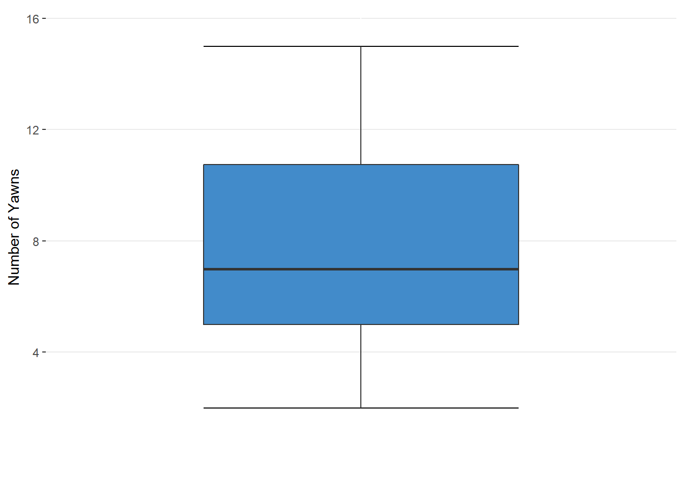 Figure 6.11. A Box-and-Whiskers Plot
Summing it Up
To describe a distribution of data, one needs to give a description of where the bulk of data are (central tendency) and how similar or variable the data are (variability). The measures of central tendency and variability appropriate for a set of data depends on the scales of measurement and the presence of skew. It is often useful to present multiple descriptive statistics in a summary or figure. These descriptive statistics for a sample will be important for forming an estimate for the population parameters.
Where We’re Going
Understanding the shape of distributions will allow us to: * Judge how many of the observations lie within a range of values + How many students will score between a 1100 and 1300 on the SAT? * Estimate the chances of getting some value from a population + Assuming men are - on average - 6 feet tall, how likely is it that we’ll get sample with an average height of 6’3“? * Decide if two samples come from the same population + Can we consider IQ scores from SVSU and GVSU students equal, on average? * Judge the likelihood that multiple samples have come from the same population + Do different brands of acetaminophine have different fever reduction times? * Determine if the relationship found in a sample is likely to be found in the population + Does the amount of time spent studying relate to college GPA?
As you may deduce, we are really setting the stage for inferential statistics by learning about the properities of distributions.
References
Wikimedia (2011). Frankfurt Citymap WTS. Retrieved May 16, 2018 from https://commons.wikimedia.org/wiki/File:Frankfurt_citymap_wts.jpg