By completing this section, you will be able to:
-
Define probability
-
Calculate simple probabilities
-
Determine appropriate probability to calculate for multiple events
-
Calculate conditional probabilities
-
Explain how probability allows for prediction and generalization
-
Create probability distributions
-
Relate mean, expected value, and population parameters
Professor Weaver’s Take
Most institutions have courses such as “Probability and Statistics” or “Probability Theory” in various departments like Mathematics, Finance, Economics, and Psychology. This course is simply titled “Statistics.” That is not too imply that probability is not important for this course; it is essential for the ability to make conclusions about populations beyond our sample. However, “probability” is not in the course title because we will only focus on probably as it pertains to the logic of generalizing from our samples. There is something valuable in understanding some of the basic principles of probability just for everyday life. If your retirement plan is to win the lottery, you may want to pay particularly close attention to this chapter.
This chapter is about related but different concepts. You’ve surely heard phrases like “what are the odds of that?” or “that seems likely” One of my favorites is “there is a thirty percent chance of rain.” In each of these, were referring to a quantification of certainty or uncertainty. Although these concepts are similar, there are important differences in how we draw a conclusion about that uncertainty. When I was in graduate school, I saw a weather man struggle with expressing these concepts. Unfortunately for this poor gentleman, the news anchor was feeling a little mischievous when he asked what it meant that there was a 50% chance of rain. The weatherman was searching for either the right answer or the right way to give his answer; neither came out. After an awkward pause and telling “um”, he started that “50% of the viewing area would get rain today.” What it really means is that it had rained half of the days that had similar conditions. Although it may have also been true on that particular day that half of geographic region experienced some rain, the process of determining this likelihood did not include a line dividing the greater Cleveland area. II reference this example because I don’t want anyone in my course to be in this unfortunate position. I don’t expect anyone to become a meteorologist but I do expect some of you to be in the business of predicting the future, like meteorologists. Meteorology is the science of predicting future weather events, as such, those in that field should understand what those predictions mean.
In addition to helping you interpret probabilities and odds when you encounter them in your everyday life, the discussion of probability will help set the stage for more important concepts to come in this course. By understanding probability, we will be able to make a judgment about the likelihood of getting a specific test statistic given our sample size and the characteristics of our sample distribution. Essentially, we will be using probability to help guide our decision-making process. When asking if the results of our statistical analyses are meaningful or useful, we will be assessing the certainty of obtaining those results. Before we get to hypothesis testing and decision making, we must get the basics under our belts. Let us start with the most basic question for this section: what is probability?
Probability
Probability is a number that represents how certain one is that an event will occur. It is represented as a proportion (between 0 and 1). An event with a probability of 0 will not occur whereas an event with a probability of 1 will occur. For example, we might reasonably assign a probability of 0 to the event of a dinosaur appearing in Time Square wearing overalls and reciting Shakespeare. However, we would sign a probability of 1 to the event of there being at least one atom of oxygen existing in your lungs as you read this.
These extreme values are not very interesting because the refer to certainty. We are more interested determining the chances of events that may or may not happen. In science and statistics, we appreciate values of 0 (never) and 1 (always) as possibilities but that most of the natural world exists in between. To determine the probability of occurrence we need to determine answers to the following questions:
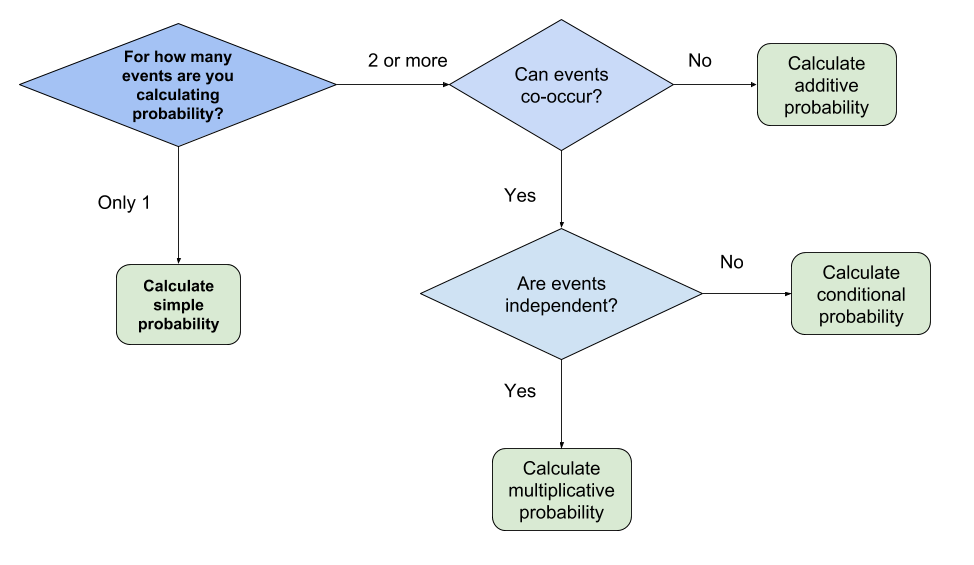
Figure 7.1. Flowchart for deciding which probability to calculate
Simple Probability
When determining the probability of a single event, you need only count and divide. Count the number of instances that match the event and divide by the number of total possible events. We can express this with the following equation for the probability of event A:
\[ p(A) = \frac{n_{A}}{N} \]
Here, p(A) is read as “the probability of A”, nA is the number of A events, and N is the total number of events.
Simple probability is the chance of some event occurring and is expressed as the proportion of the number of times that event occurs by the total number of events.
Let’s with through an example in which you are determining the probability of randomly selecting a green Skittles from a new bag. Let’s assume that the Skittles website reports (I checked and this information does not exist) that each 5-ounce bag contains the following colors and quantities:
Table 7.1
Color and quantities of Skittles
| Color | Quantity |
|---|---|
| Purple | 9 |
| Green | 10 |
| Yellow | 12 |
| Orange | 11 |
| Red | 8 |
Given this, we know our bag will contain 10 green Skittles and a total of 50 Skittles. If we insert these values into our formula, we get
\[ p(\text{Green}) = \frac{n_{\text{Green}}}{N} = \frac{10}{50} = 0.20 \]
The probability of pulling out a green Skittles from our new bag is 0.20. That is 20% of the Skittles we take out of the bag should be green.
We need to check some expectations about probabilities before continuing. The probability of some event occurring is really the probability of the event occurring in the long-term. That is, we shouldn’t necessarily expect that 20% of the first five Skittles we pull will be green. The probability reflects what we should expect as our sampling of events (n) reaches the population (N). Cautions addressed, knowing that, we should expect about 20% of the Skittle to be Green, in the long-run, is more helpful than having no information about the probabilities of each color in the bag.
In addition to expressing probability as a percentage and a proportion, we can state it as a fraction by saying that we have a 1/5 chance of picking out a green Skittles. Expressing probability as fraction allows you to easy convert this statement to statistical odds. Statistical odds reflect the ratio of successes (events that you are interested in) to failures (any other event).
We need to tweak our probability fraction slightly. As it stands, the fraction represents the number of successes relative to total number of events. We need to determine the relative number of failures for the denominator. This is done by subtracting the number of success from the total number of events. That is, nfailure = N – nsuccess. We now have that for every 1 success, we can expect 5-1 = 4 failures.
Now that we have our relative counts, we can express them as an odds ratio. We would state that the odds of selecting a green skittles are 1:4. Remember, this is expressing something slightly different than our simple probability. The simple probability reflects the ratio of a success to all possible events whereas odds represent the ratio of success to failures. You can phrased. Probabilities are usually expressed with the word “in” whereas odds are usually spot the difference between probability and odds by the way it is usually expressed with the word “to.” For example, “the chances of winning are 1 in 5” states the probability whereas “the odds of winning are 1 to 4.”
Probability of Multiple Events
Knowing the simple probability of one event is helpful but we are often more interested in the complex occurrence of multiple events. Let’s revisit the Skittles bag for a moment by adding a few more variables to our dataset. In addition to the color, let’s indicate the flavor and our preferences for flavor and color.
Table 7.2
Flavors, Colors, and Preferences for Skittles
| Like Flavor | Flavor | Like Color | Color | Quantity |
|---|---|---|---|---|
| No | Grape | Yes | Purple | 9 |
| No | Green Apple | Yes | Green | 10 |
| Yes | Lemon | Yes | Yellow | 12 |
| Yes | Orange | No | Orange | 11 |
| Yes | Strawberry | No | Red | 8 |
As indicated in the probability flowchart (figure 7.1), we need to decide if events can co-occur.
Mutually Exclusive Events
If we draw just one Skittles, it can only have one value per variable. That is, any Skittles can have just one flavor and just one color. We may like or dislike the color or flavor. We cannot draw a purple and green Skittles. Therefore, color and flavor are mutually exclusive events for each skittle. Similarly, the number that comes up on a die or the side that comes up on a coin flip are mutually exclusive events. We can represent the relationship of these events using a Venn Diagram (see figure 7.2).
Mutually exclusive events cannot co-occur.

Figure 7.2. Venn diagram of mutually exclusive color events when choosing one Skittles
Because we cannot calculate the probability of one Skittles being both green AND purple, we will have to determine the probability of a Skittles being green OR purple. To determine the probability of mutually exclusive events, you simply add together the probabilities of each event. The formula is:
\[ p(\text{A or B}) = p(A) + p(B) \]
Let’s calculate the probability of drawing a Skittles from the bag that is green or purple by first calculating the simple probabilities of each.
\[ p(\text{Green}) = \frac{n_{\text{Green}}}{N} = \frac{10}{50} = 0.20 \]
\[ p(\text{Purple}) = \frac{n_{\text{Purple}}}{N} = \frac{9}{50} = 0.18 \]
Now we can add those two probabilities together
\[ p(\text{Green or Purple}) = p(\text{Green}) + \ p(\text{Purple}) = 0.20 + 0.18 = 0.38 \]
That is, on any random draw from our full bag, we have a 38% chance of selecting a green or purple Skittles.
Independent Events
What if we want to draw more than one Skittles? If we draw two Skittles from two bags, each Skittles can have its own set of values. That is, Skittles A can be purple and Skittles B can be green. Importantly, these are independent events because the color of the first Skittles does not impact the color of the second Skittles. If we draw from the same bag and don’t replace our first draw, it changes the counts and thus the probabilities of the remaining draws.This makes the probability of sequential draws dependent previous draws. We’ll cover this in the next section.
Independent events do not affect the probability of one another.
Determining the probability of independent events, we need to multiply the simple probabilities of the events. Recall that probability is a number between 0 and 1. Because we are multiplying two decimals, the product (result) must also be a decimal between 0 and 1 and will be less than either of the two factors. Apart from the mathematics, you can visualize why the probability of two independent events is less than the either of the two simple probabilities. Rather than simply looking at the number of Skittles in a bag, we are looking at the total possible combinations of all the Skittles across two bags. Out of these, we want to know how many match the purple and green combination in a draw from each bag. Figure 7.3 shows an excerpt of all the possible combinations.
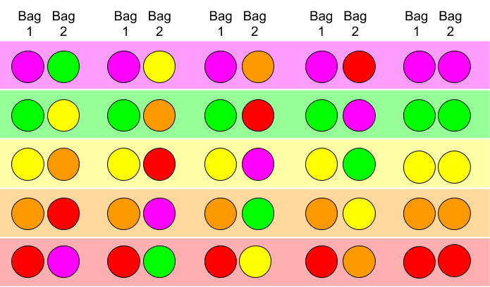
Figure 7.3 A sample of possible skittles combinations across two draws from two bags.
Dependent Events
It is interesting and necessary to know about individual variables but we are more often interested in how two or more variables are related. This will be the bulk of the statistical tests that we will explore in this course. It is often the case that a change in the value of one variable impacts the value of another. This is true for probability when we examine the probability of observing an event given the value of some other variable. Let’s examine this using our Skittles dataset.
| Like Flavor | Flavor | Like Color | Color | Quantity |
|---|---|---|---|---|
| No | Grape | Yes | Purple | 9 |
| No | Green Apple | Yes | Green | 10 |
| Yes | Lemon | Yes | Yellow | 12 |
| Yes | Orange | No | Orange | 11 |
| Yes | Strawberry | No | Red | 8 |
There is overlap in the preferences for flavor and color. It may be easier to see if we change the format of the table. Table 7.3 shows which Skittles fall into the combination of the preference variables.
Table 7.3
Restructured Table of Skittles Data
| Like flavor | Do not like flavor | |
|---|---|---|
| Like color | Yellow / lemon (12) | Purple / grape (9) |
| Green / green apple (10) | ||
| Do not like color | Orange / orange (11) | |
| Red / Strawberry (8) |
This view makes it easier to notice that there is clearly some overlap between preferred colors and flavors. As such, we can not calculate the probability of selecting a color and flavor that we like as a product of the two simple probabilities. Instead, we will need to calculate the conditional probability. This means the probability of observing a value for one variable depends on the value of another variable. To help us see this relationship, let us further simplify or table by collapsing (removing the different values of) flavor and color so that we just retain the number of Skittles that for into each cell. We will also add in the marginal totals, which are the total number of observations in each column our row.
conditional probability involves determining the how the occurence of one event impacts the probability of another event.
Table 7.4
Collapsed Counts of Skittles for Preferences with Marginal Totals
| Like flavor | Do not like flavor | Total | |
|---|---|---|---|
| Like color | 12 | 19 | 31 |
| Do not like color | 19 | 0 | 19 |
| Total | 31 | 19 | 50 |
To determine the probability of any of the combination of events (i.e., one of the cells in the table), you divide the count for that cell by the grand total (N = 50). For example, the probability of selecting a Skittles that has a color and a flavor that are liked is:
\[ p(\text{like flavor and color}) = \frac{n_{\text{like flavor and color}}}{N} = \frac{12}{50} = 0.24 \]
If we assumed that the events were independent and used the multiplicative rule, we would have found that:
\[ p(\text{like flavor and color}) = p(\text{like flavor})*p(\text{like color}) = \frac{n_{\text{like flavor}}}{N}*\frac{n_{\text{like color}}}{N} = \frac{12 + 19}{50}*\frac{12 + 19}{50} = \frac{31}{50}*\frac{31}{50} = 0.38 \]
The incorrect assumption of independence overestimates the probability the co-occurrence of non-independence of events.
Conditional Probability
With dependent events, we can ask more directed questions. Rather than asking about the chances of selecting a Skittles that has a flavor and color we like, we can restrict our sample by one of the characteristics.
For example, we could separate the bag of Skittles into colors we like (purple, green and yellow) from those we do not like (orange and red). We can then ask about the probability of selecting flavors we like from each of these. We could state this as, “given that I have colors I like, what is the probability of selecting a Skittles with a flavor I like.” The short-hand notation for this is “ p(B | A)” where the “|” or vertical bar indicates the conditional probability of event B, given that event A has occurred. In our example, we assume that event A (selecting only those Skittles with the colors we like) has already occurred. This then limits our selections for event B (getting a Skittles with a flavor we also like).
The process of finding the conditional probability is quite easy if you have a table such as 7.4. The first step is to highlight the row or column that corresponds to the “given” statement. In our case, we are only interested in the Skittles with Colors we like, so we will focus on the first row.
| Like flavor | Do not like flavor | Total | |
|---|---|---|---|
| Like color | 12 | 19 | 31 |
| Do not like color | 19 | 0 | 19 |
| Total | 31 | 19 | 50 |
Once we’ve restricted our table, we determine the simple probability of getting a flavor we like by dividing the count of “like flavor” by the marginal total for “like color”.
\[ p(\text{Like Flavor | Like Color}) = \frac{n_{\text{like flavor within like color}}}{n_{\text{total like color}}} = \frac{12}{31} = 0.387 \approx 0.39 \]
That is, once we’ve selected the colors we like, we have a 39% chance of selecting a Skittles with a flavor we also like.
The implications for conditional probabilities of dependent events goes beyond the scope of this course (check out this overview of Bayesian Statistics). For now, we’ll appreciate that we can represent the dependence of some outcome on the status of some other variable.
Probability Distributions
So far, we’ve been discussing how to determine the chances of observing some possible event. That is, we have calculated the probability of each potential value of a variable occurring in some dataset. If you felt a sense of Déjà vu, it is because we had covered this procedure in the previous module, using a different name. The probability of each value for a variable was expressed in the relative frequency distribution. Table 7.6 shows the relationship between the count of various colors of Skittles (table 7.1) and the relative frequency distribution for that information
Table 7.6
Relative Frequency Distribution for Skittles Colors
| Color | Quantity | Relative Frequency |
|---|---|---|
| Purple | 9 | = 9/50 = 0.18 |
| Green | 10 | = 10/50 = 0.20 |
| Yellow | 12 | = 12/50 = 0.24 |
| Orange | 11 | = 11/50 = 0.22 |
| Red | 8 | = 8/50 = 0.16 |
As you may recall, the relative frequency is the simple frequency of the value divided by the total number of observations. This is the same formula as simple probability. As such, a probability distribution expresses the chances of observing each possible value of a variable.
A probability distribution contains each possible value and the probability of observing each value
Although the information in a relative frequency distribution and a probability distribution are the same, a probability distribution is written in horizontal format.
Table 7.7
A Probability Distribution of Skittles Colors.
| Color of Skittles | ||||||||||
|---|---|---|---|---|---|---|---|---|---|---|
| Purple | Green | Yellow | Orange | Red | Σ p(x) | |||||
| p(x) | .18 | .20 | .24 | .22 | .16 | 1.00 | ||||
Our table includes all of the possible colors, or 100%, of the Skittles. As such, our probabilities should add up to be 1.00. That is, we have a 100% of selecting a purple, green, yellow, orange or red Skittles.
The benefits of expressing counts as relative frequency or probability are two-fold.
-
We can express the distribution in general terms. That is, we can indicate the proportion of the total sample falling into each value or category without having to reference the actual counts. This allows for easy comparison across different samples.
-
Knowing that probability indicates the chances of observing events in the long-run, we can express the likelihood of some value in any for any sample. This gives us some grounds for prediction and estimation of population parameters.
Expected Value
Let us add in a few more previously discussed components: central tendency and variability. Just as we were able to calculate the mean and standard deviation of a distribution by using all of the values in the dataset, we can use the generalized probabilities to calculate the mean of a probability distribution. The mean of a probability distribution has a special name, the expected value (µ). The expected value is the average value we should expect to find over many observations. “µ” is the Greek symbol “mu,” which is used to represent the population mean.
The expected value (µ) the average value of many observations.
What is the expected value for the color of Skittles drawn at random? If you guessed “yellow,” you have the right mind for statistical analysis. However, the correct answer is “not applicable.” Let me explain. There is no expected value (as we’ve defined it) because you cannot calculate the mean for nominal scales of measurement (in this case, color). That being said, the value you might expect to find is the one with the highest probability. We just equated probability with relative frequency. Therefore, the value with the highest probability is the mode of the probability distribution and is thus the correct value of central tendency for nominal data. Thinking like a statistician does not only mean knowing the definitions, but it means that you need to have an appreciation for the core questions (e.g., What is the best way to describe this? What is my best estimate for this data?).
To demonstrate how to calculate an expected value, we must move to ordinal, interval, and ratio scales of measurement. Sticking with our Skittles theme, table 7.8 represents the probabilities of selecting an individual who has eaten 1, 2, 3, 4 or 5 bags of Skittles in the last month.
Table 7.8
Probability Distribution of Skittles Ratings
| Number of bags of Skittles a | ||||||||||
|---|---|---|---|---|---|---|---|---|---|---|
| 1 | 2 | 3 | 4 | 5 | Σ p(x) | |||||
| p(x) | .15 | .21 | .25 | .22 | .17 | 1.00 | ||||
Note. a Consumed in last six months
The easiest way to calculate the expected value is to use the following formula:
\[ E(x) = \mu = \sum_{}^{}{x*p(x)} \]
Translated into English, this formula states that the expected value (µ) is equal to the sum of the product of each value times the probability of that value.
We can break it down into steps.
Step 1: Multiply the value by the probability
| Number of bags of Skittles | ||||||||||
|---|---|---|---|---|---|---|---|---|---|---|
| 1 | 2 | 3 | 4 | 5 | Σ | |||||
| p(x) | .15 | .21 | .25 | .22 | .17 | 1.00 | ||||
| x* p(x) | .15 | .42 | .75 | .88 | .85 | |||||
Step 2: Add up the products
| Number of bags of Skittles | ||||||||||
|---|---|---|---|---|---|---|---|---|---|---|
| 1 | 2 | 3 | 4 | 5 | Σ | |||||
| p(x) | .15 | .21 | .25 | .22 | .17 | 1.00 | ||||
| x* p(x ) | .15 | .42 | .75 | .88 | .85 | 3.05 | ||||
For our example, the expected value (µ) of the number of bags of Skittles consumed in the last month is 3.05 bags. Notice, no one reported eating fractions of bags. As such, you should interpret expected value as the expected average value of any such distribution.
The magic of this formula is that we weight each value by the probability rather than including all the observations that have each value.
Standard Deviation
The description of a distribution needs a measure of variability to compliment that of central tendency. We will calculate variance / standard deviation to compliment the mean of the probability distribution. Just as we weighted the values of our distribution with their respective probabilities, we will weigh the deviation of values from the mean by each values probability.
\[ \sigma^{2} = \sum_{}^{}{\left( x - \mu \right)^{2}*p(x)} \]
This formula states that the population variance (σ2, lower-case sigma squared) is equal to the sum of the squared difference between each value and the mean multiplied by the probability of each value. Let’s complete this in steps.
Step 1: Calculate difference between each value and mean (µ)
| Number of bags of Skittles | ||||||||||
|---|---|---|---|---|---|---|---|---|---|---|
| 1 | 2 | 3 | 4 | 5 | Σ | |||||
| x- µ | 1-3.05 = -2.05 | 2-3.05 = - 1.05 | 3-3.05 = -0.05 | 4-3.05 = 0.95 | 5-3.05 = 1.95 | |||||
Step 2: Square the difference
| Number of bags of Skittles | ||||||||||
|---|---|---|---|---|---|---|---|---|---|---|
| 1 | 2 | 3 | 4 | 5 | Σ | |||||
| x- µ | 1-3.05 = -2.05 | 2-3.05 = - 1.05 | 3-3.05 = -0.05 | 4-3.05 = 0.95 | 5-3.05 = 1.95 | |||||
| (x- µ) 2 | 4.2025 | 1.1025 | 0.0025 | 0.9025 | 3.8025 | |||||
Step 3: Multiply the squared differences by the probability
| Number of bags of Skittles | ||||||||||
|---|---|---|---|---|---|---|---|---|---|---|
| 1 | 2 | 3 | 4 | 5 | Σ | |||||
| x- µ | 1-3.05 = -2.05 | 2-3.05 = - 1.05 | 3-3.05 = -0.05 | 4-3.05 = 0.95 | 5-3.05 = 1.95 | |||||
| (x- µ) 2 | 4.2025 | 1.1025 | 0.0025 | 0.9025 | 3.8025 | |||||
| p(x) | .15 | .21 | .25 | .22 | .17 | |||||
| (x- µ) 2* p(x) | 0.630 | 0.232 | 0.001 | 0.199 | 0.646 | |||||
Step 4: Add up the products
| Number of bags of Skittles | ||||||||||
|---|---|---|---|---|---|---|---|---|---|---|
| 1 | 2 | 3 | 4 | 5 | Σ | |||||
| x- µ | 1-3.05 = -2.05 | 2-3.05 = - 1.05 | 3-3.05 = -0.05 | 4-3.05 = 0.95 | 5-3.05 = 1.95 | |||||
| (x- µ) 2 | 4.2025 | 1.1025 | 0.0025 | 0.9025 | 3.8025 | |||||
| p(x) | .15 | .21 | .25 | .22 | .17 | |||||
| (x- µ) 2* p(x) | 0.630 | 0.232 | 0.001 | 0.199 | 0.646 | 1.708 | ||||
The variance of the probability is 1.708 bags of Skittles squared. Of course, it’s easier to wrap our minds around standard deviation (σ) because it is in the same units as the variable. To determine the standard deviation, simply take the square root of variance. For our example, the standard deviation is 1.307.
Summing it Up
Probability is the chance of making observing a particular value of a variable. This is expressed as a proportion between 0 and 1. The probability can be simple (one event) or may require some consideration of multiple events. When the events are mutually exclusive, one can simply add together the individual probabilities. If multiple events co-occur but are independent, the probabilities need to be multiplied. Lastly, if multiple events co-occur but are not independent, one must calculate the conditional probabilities.
Once the probabilities are established, the probabilties of events can be summarized as a probability distribution. The mean of these distributions are the expected value for the variable. That is, once we know the probabilities of each possible value of a variable, we can determine the value that we should expect to find, in the long run.
Where we are going
We’ve been describing the chances of observing a particular value of a variable or the chances of observing the combination of multiple events. This is interesting enough for making decisions when gambling but there is a bigger picture with which we should be concerned. We will soon start discussing inferential statistics in which we will be determining estimates for populations based off of our samples (like we had done with the expected value of a probability distribution) and making a judgement regarding the statistical significance of those estimates. In essence, we will be making a judgement of how likely it would be to get such a parameters under certain assumptions.
We still have a few more important concepts to cover before we can get to that transition but we are very close!
Please complete and submit the homework for this section before taking the quiz.