By completing this section, you will be able to:
- Explain the characteristics of the family of normal distributions
- Relate the Empirical Rule to probability, mean, and standard deviation
- Calculate z-scores from raw scores
- Identify the probability of obtaining z-scores using the Standard Normal Distribution
Professor Weaver’s Take
Humans love to make comparisons. In fact, one might argue that no matter what we’re doing, we are comparing it to some other experience or idea. Perhaps you are grocery shopping. You may wonder if it is a good price on the coffee you’re considering. Maybe you’re thinking that you’re wanting a long time at checkout on this visit. In either case, you need the context of other observations (e.g., price of that coffee at other stores, wait time on other visits). If you have access to that data, you can determine the relative expense or duration perhaps by determining the percentile of your observation. As we’ll learn in this chapter, we can easily determine the likelihood of observing a range of values of those values approximate a normal distribution.
The Family of Normal Distributions
As discussed previously, a normal distribution is symmetrical about the peak, with the peak representing the mean, median, and mode. The particular values of central tendency can be any value (-∞, +∞) because any continuous variable could theoretically be normally distributed and there are no limits to the values that variables can have. The variance of normal distributions can likewise be any value greater than 0. All this is to indicate that “the normal distribution” is a bit of a misnomer. It is better to describe the family of normal distributions, each member of which is defined by its mean and standard deviation. The notation is N (M,s) where “N” indicates “normal”, “M” is the mean and “s” is the standard deviation. Figure 8.1 presents some normal distributions.
A normal distribution is symmetrical about the mean with the tails exteneding to +/- ∞.
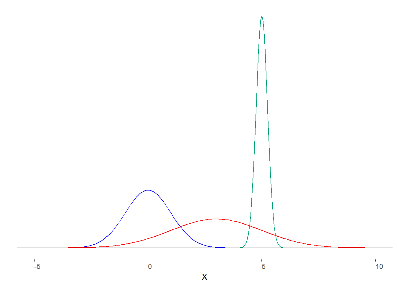
Figure 8.1. Several normal distributions.
Apart from their symmetry, each of these distributions share a important characteristic. They are histograms that represent the relative frequency of the values. This means that the normal distribution can also tell is about probability.
Area Under the Curve
All normal distributions are also probability distributions. They can tell is the probability of getting a range of values but not the probability of obtaining an exact value. The mathematical reason requires some understanding of integral calculus. We won’t assume that requirement for this course. Instead, let us borrow one important concept from calculus, the area under the curve. Roughly speaking, the area under the curve of the normal distribution equals the probability of obtaining values associated with the upper and lower bounds of the curve. If we look at the whole curve, the area under the curve is 100% or 1.00. This means that we have a100% chance of observing any value. If we restrict the curve to just the top half, we would know that we have a 50% chance of observing a value above the mean. What if we restrict to just the value of the mean? It seems that there is good reason to suspect a higher likelihood of observing the mean because it is also the mode (most frequently occurring value). However, the area under the curve for one exact value for a continuous variable is essentially zero! What nonsense! Here’s the trick: there is no distance between the mean and the mean. Therefore, there can be no area associated with a distance of zero. Do not fret as statisticians do not work in exact values. We are much more comfortable with intervals and confidence ratings.
The area under the curve for a range is equal to the proportion of scores in that range
The Empirical Rule
What use is the normal distribution if we can’t know the probability of exact values? We can easily judge the probability of ranges of values if we know the mean and standard deviation of the distribution. No matter what the parameters of the normal distribution, we know that 68% of observation will fall between a standard deviation below the mean and a standard deviation above the mean. Between two standard deviations above and below the mean lie 95% of the data. Finally, 99.7% of observations are between 3 standard deviations below the mean and 3 standard deviations above the mean. Figure 8.2 represents these relationships.
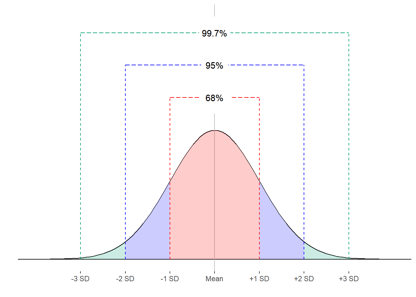
Figure 8.2. The empirical rule and the normal distribution.
Because area under the checked equates to an estimate of probability, we can also say that we have a 68%, 95% and 99.7% chance of making an observation between 1, 2 and 3 standard deviations around the mean, respectively.
Also, recall that the area under the curve is equal to 1.00. This means that the proportion of observations more extreme than 3 standard deviation away from the mean is 1.00 – 0.997 = 0.003. That’s a very unlikely occurrence. Not impossible but unlikely. It is so unlikely that we may consider values that are beyond 3 standard deviations of the mean to be from a different distribution all together. This is an important concept that will be with us for statistical hypothesis testing.
The Z-transformation and the Standard Normal Distribution.
One of the benefits for focusing on the family of normal distributions is that you can compare values within a distribution and across other normal distributions. To can compare scores within a distribution by simply comparing the raw scores, which are in the original units of the measure. If you want to compare across normal distributions, you need to put the various scales into a common metric. That is, you can’t readily decide if 176 pounds is more likely than having an IQ of 112. Luckily for us, we can convert any normally distributed variable into an easy to compare metric in two steps. We will perform the Z-transformation to change raw scores into standard deviation scores or z-scores. What I mean is that we will refer to how many standard deviations away from the mean a score is rather than it’s value in units. Because we know about the normal distribution and the empirical rule, we can easily compare two scores that are expressed in standard deviations.
Raw scores are those that are in the units of the original data.
Z-scores are transformed scores representing the number of standard deviations a raw score is from the mean of the distribution.
Performing the Z-transformation
Let’s turn a test score into a z-score. We’ll assume that the mean for the class was 0.78 with a standard deviation of 0.07. We’ll transform a score of 0.82 into a z-score by following these steps.
STEP 1: Subtract the mean from the score
Difference = 0.82 – 0.78 = 0.04
STEP 2: Divide difference by standard deviation
\[ z = \frac{\text{difference}}{\text{standard deviation}} = \frac{0.04}{0.07} = 0.57 \]
The full formula is
\[ z = \frac{x - M}{s} = \frac{0.82 - 0.78}{.07} = 0.57 \]
Where x is the raw score, M is the mean, and s is the standard deviation. Remember that our new unit for the z-scores is standard deviations, so an exam score of 82% is 0.57 standard deviations above the mean for the class.
Standard Normal Distribution
When you use this formula to convert scores to z-scores, you are transforming your distribution into the Standard Normal Distribution. This is a very special member of the normal distribution family because the mean is 0 and the standard deviation is 1. It is nice to convert scores to this Standard Normal Distribution because someone has already done the calculus for us to determine the area below the curve for different ranges of z-scores. You can find a table of z-scores and associated proportions of scores in the Unit Normal Table (z-table). Figure 8.3 is an excerpt from this larger table.
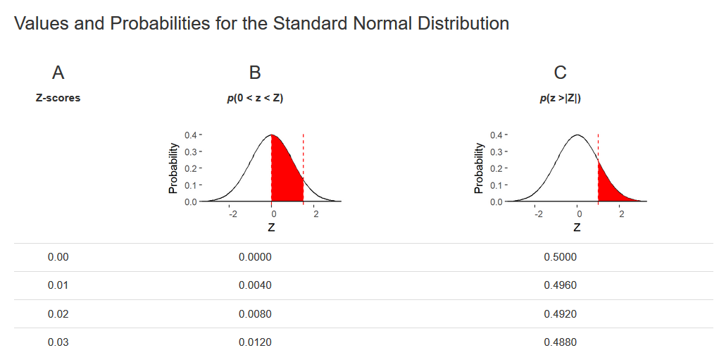
Figure 8.3. Exceprt from Unit Normal Table
Notice the columnar layout of the table. Column A contains the z-scores starting at 0 and continuing to 4. There are only positive z-scores in this table because of the symmetrical nature of the normal distribution. If you want to know about a negative z-score, consult the absolute value of that score in the table. Column B contains the proportion of observations between the z-score and the mean. We might refer to this as the body of the distribution. Column C contains the proportion of scores more extreme than the z-score. This is often referred to as the tail of the distribution.
Let’s find a few common values in this table. A z-score of 0 has a value of 0.0000 for column B and 0.5000 for column C. Why is this? To get a z-score of 0, the raw score must equal the mean. There is no distance between the mean and itself so there are no scores between the mean and itself. Why does column C have a value of 0.50? Recall that the mean is equal to the median and the mode for the normal distribution and that the median is the 50% point or 50th percentile of the distribution.
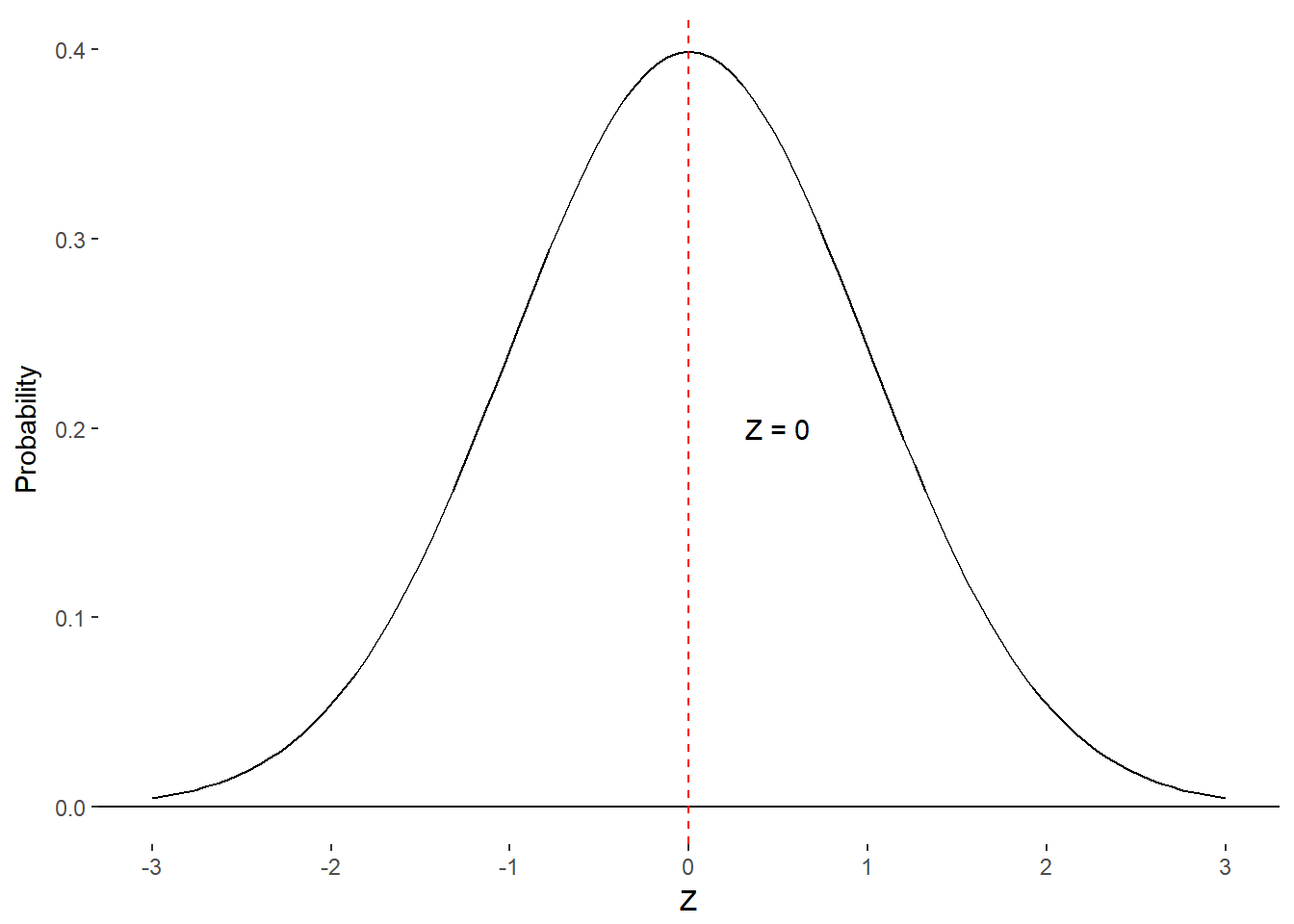
Figure 8.4. proportion of scores associated with z = 0.
According to the empirical rule, 68% of the observation should fall between 1 standard deviation below the mean and 1 standard deviation above the mean. Consulting the table, we find a value of 0.3413 for column B. Why does this seem different from the empirical rule? Recall that column B is only between the mean and the z-score and the empirical rule includes both sides of the distribution. We can rectify these two representations by simply multiplying column B by 2. Similarly, you will find a value of 0.4772 in column B for a z-score of 2. If we multiply column B by 2, we get 0.9544, which corresponds to the 95% described by the empirical rule.
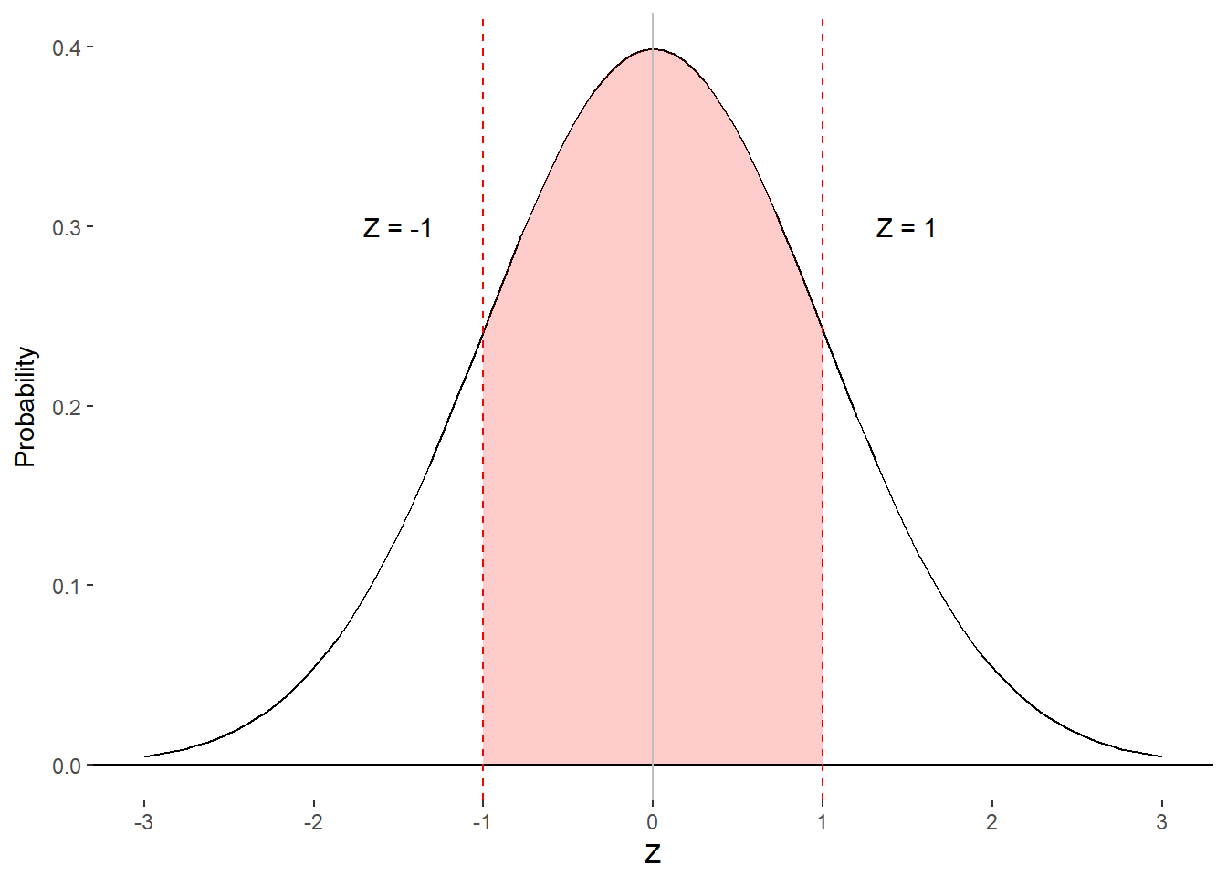
Figure 8.5. proportion of scores associated with z = 1 and z = 2.
Now let’s explore column C. As a rule, column C + column B = 0.5000. This is the case because the area under the right half of the distribution is 0.5000 and the z-score divides that half into columns B and C. As such, column C is a little redundant with column B but is included for convenience. For example, we may wish to know what z-score corresponds to the cut-off for the top 10% of observations. In this case, it makes intuitive sense to look in column C for a value close to 0.1000. The closest we can find is 0.1003, which corresponds to a z-score of 1.28 in column A.
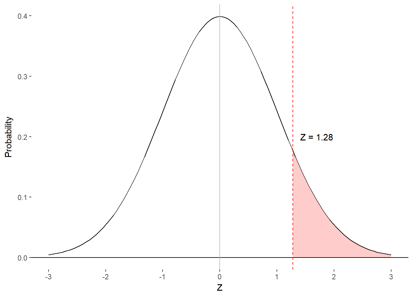
Figure 8.6. z-score associated with top 10% of scores.
We’ve been focusing on finding the proportion of scores more extreme than a z-score (column C), the proportion of scores between a z-score and the mean (column B) and the z-score associated with a certain proportion of scores (column A). Let’s show the power of the Standard Normal Distribution by determining the proportion of scores associated with different ranges of z-scores.
Both Scores on Same Side of the Mean
Let’s revisit the exam scenario and assume you want to know what proportion of scores are between 95% and 85%. We’ll first have to convert these scores to z-scores.
\[ z = \frac{x - M}{s} = \frac{.95 - .78}{.07} = \frac{.17}{.07} = 2.43 \]
\[ z = \frac{x - M}{s} = \frac{.85 - .78}{.07} = \frac{.07}{.07} = 1.00 \]
We need to find the proportion of scores that are between 1.00 and 2.43 standard deviations. We have two options. One of them is not to look up values associated with the difference of the two z-scores. Remember, we need to find the area under the curve between these two values.
Option 1: Subtract Column Bs
We can find the area under the curve between these two z-scores by subtracting the value in column B for the smaller z-score from the value in column B for the larger z-score.
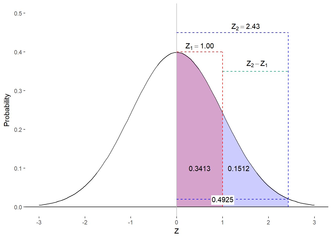
Figure 8.7. Finding proportion of scores in range using column Bs
Column B yields 0.4925 for a z-score of 2.43 and 0.3413 for z=1.00. Through subtraction, we find the proportion of scores between exam scores of 95% and 85% is
\[ 0.4925 - 0.3413 = 0.1512 \]
That is, we can expect around 15% of individuals to score between an 85% and 95%.
Option 2: Subtract Column Cs
If you want, you can focus on the difference in the tails rather than the body of the distribution by using column C. In this case, you will subtract the value in column C for the larger z-score from the value in column C for the smaller z-score.
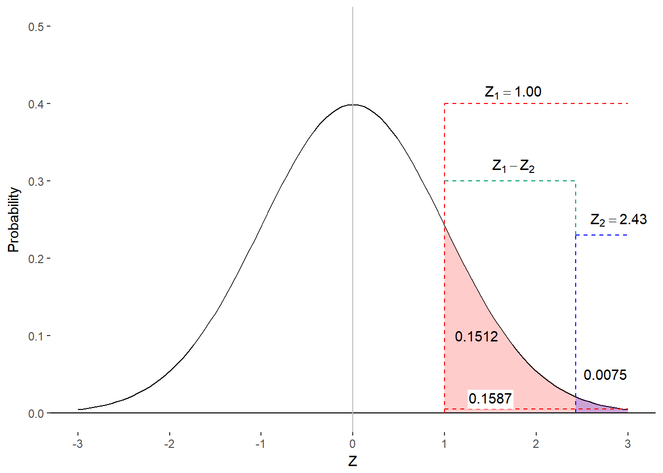
Figure 8.8 Finding proportion of scores in range using column C
We find the following values in column C for z = 1.00 and z = 2.43, respectively: 0.1587 and 0.0075. Once again, we find that
\[ 0.1587 - 0.0075 = 0.1512 \]
Scores on Opposite Sides of the Mean
Now let’s assume that were interested in the proportion of students that scored between 65% and 83%. We will need to convert those scores to z-scores just as we did before.
\[ z = \frac{x - M}{s} = \frac{.83 - .78}{.07} = \frac{.05}{.07} = 0.71 \]
\[ z = \frac{x - M}{s} = \frac{.65 - .78}{.07} = \frac{- .13}{.07} = - 1.86 \]
Notice that the lower score yields a negative z-score because it is below the mean. We will not find any negative values in our table. No worries, we will just consult the table for the absolute value (i.e., the positive version) of our negative z-score but we will have to remember that it is actually representing proportion of scores below the mean.
We want to know the proportion of scores between these two values but we do not have a direct way of getting that information from the table. Instead, we will have to build that value from two. Figure 8.7 identifies the z-scores on the Standard Normal Distribution and the areas under the curve with which we are concerned. Once we’ve mapped out the information on the histogram, we can see that column B contains the relevant information. We can determine the proportion of scores between z = -1.86 and z=0.71 by adding together their corresponding values from column B. A quick check of our table tell us that 0.2611 of scores are between 0.71 and the mean and that 0.4686 of scores are between 1.86 and the mean. Adding these scores together, we get
\[ 0.2611 + 0.4686 = 0.7297 \]
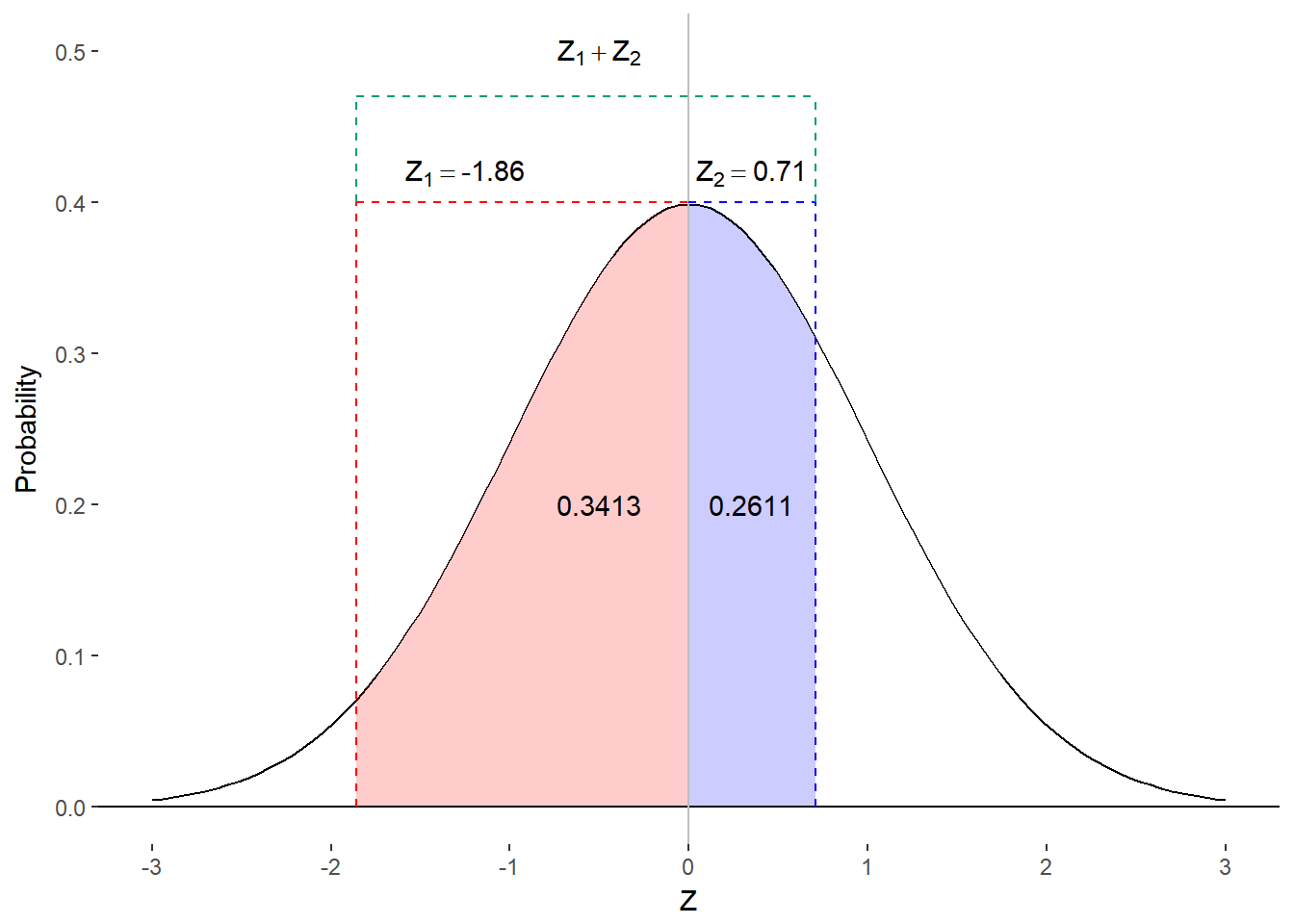
Figure 8.9. Finding proportion of scores on opposite sides of the Mean
Nearly 73% of students scored between 65% and 83%.
Given any score, we can find the proportion of scores above, below, or between that score and the mean (providing the scores are normally distributed). If we have two scores, we can find the proportion of scores that lie between those values.
Summing It Up
The family of normal distributions are very useful in statistical analyses because of their presence in many phenenomena as well as their regular structure. That is, all normal distributions can be transformed into the Standard Normal distribution that has a mean of 0 and a standard deviation of 1. Any score from a normal distirbution can be represented as a z-score on the standard normal distribution by using simple formula:
\[ z=\frac{x-M}{s} \] The z-score is thus a representation of how many standard deviations a raw score is from the raw mean. Having this information, we can look up the area under the curve (i.e., proportion of scores) relative to this score using the Unit Normal Table. We can find the proportion of values that are more extreme than the z-score, the proportion between the z-score and the mean, or the proportion between any two z-scores.
Where We’re Going
There are many phenomena that approximate normal distributions. This is one reason why statisticians have focused so heavily on the normal distribution. Perhaps another and more impactful reason for the reliance on the normal distribution is that we can easily compare various normal distributions by converting raw scores to z-scores. Furthermore, we can determine the proportion of scores above, below, or in between scores.
The ability to determine the proportion of (or probability of obtaining) scores related to some critical value will be immensely important in statistical hypothesis testing. Recall that one of the main goals of statistical analyses is to make an inference about a population given some sample data. Although it can be quite easy to conjure a guess as to the values in a population, we must also consider the amount of error (e.g., variability) in our guesses and the probability that a guess may be incorrect. We will rely quite heavily on the properties of the normal distribution that we’ve learned here as the basis for those estimates.
We have just one more important topic to cover before we can start statistical inference. So far, we have been determining the probabilities and proportions associated with values in a sample. We are not often interested in one score from a sample but rather we focus on the mean of samples. That is, we consider the mean to be a better guess for what is happening in the population than any one score from the sample. As such, we will have transition from distributions of individual scores to distributions of sample means.
Try out the homework problems by clicking “Next” below. After submitting the homework, you can take the quiz.