By completing this section, you will be able to:
- Explain the link between sample statistics, sampling distributions and population parameters
- Construct a sampling distribution of sample means and of sample variances
- Compare the standard error of the mean (SEM) to standard deviation (s)
- Explain the central limit theorem and how it used for non-normal samples
Professor Weaver’s Take
It may be hard to believe, but I’m a Millennial. It’s true that I was in the first batch but my age places me within that generation. I’ve enjoyed growing up with computers, the Internet and generally being overly concerned with myself and entitled. Although these are often used as key characteristics for Millennials, I don’t feel that the latter two apply to me. It is almost as if researchers were assessing a different group or subgroup than the one to which I belong. But how can this be? If I am a Millennial, shouldn’t my characteristics be reflected in those descriptions? There are a few processes at work here. There may be poor sampling of the population of Millennials such that my group is not included. There is definitely summarization, which implies simplification. As we’ll find out in this section, estimates about a population are built from samples and some important logic.
Sampling Distributions of Sample Statistics
Although researchers do their best to have a representative sample from the population of interest, the sample selected is only one of many possible samples. The data obtained from that sample may be very different from another. How many different values might we obtain from these various samples? Which obtained value is best representative of the population? We can answer these questions via a little demonstration.
Let’s imagine that you want to know the number of hours your fellow students spend at work each week. To better illustrate the link between sampling distributions of sample statistics and population parameters, we’ll make some assumptions. First, we need a small population (for reason’s you’ll appreciate soon) so we will assume that there are three classmates. Second, we’ll assume that someone has already asked each of your classmates but won’t share the information with you. Here is the data.
Table 9.1
Hours of Work for Small Population
| Person | Hours |
|---|---|
| A | 20 |
| B | 13 |
| C | 7 |
Third, each time you send out an anonymous survey to your classmates, only two of them respond. As such, you won’t know who you’ve asked and if you’ve asked them before. To be sure that you’ve gotten everyone in your study, you send out the survey many times. Table 9.2 outlines all of the possible combinations of groups of two students possible.
Table 9.2
Possible Combinations of Students
| A | B | C | |
|---|---|---|---|
| A | A,A | B,A | C,A |
| B | A,B | B,B | C,B |
| C | A,C | B,C | C,C |
There are 9 possible combinations of the three different. Wait, we’re counting each person’s data multiple times. That doesn’t seem right. We should discuss this before moving on.
Sampling Strategies
Depending on your goal, you can choose an experimental sampling strategy or a theoretical sampling strategy. Table 9.3 highlights two important differences.
Table 9.3
Differences between Sampling Strategies
| Theoretical | Experimental |
|---|---|
| Replace after sampling | No replacement after sampling |
| Order Matters | Order doesn’t matter |
In an experimental setting, you would not want to assess the same individual multiple times in a sample because that would bias your sample toward that individual. This means that we would not replace the sampled individuals into our population for the next assessment.
In our example, we are developing a sampling distribution, which is a theoretical distribution. To ensure that each event has an equal chance of being selected, we must keep the sample space the same size for each sample. Think of it this way, the chances of selecting any card from a full deck is 1 in 52 or 0.0192. What is the probability of selecting any other card on the next draw? That depends, if you replace the first card, the probability doesn’t change: it is still 1 in 52 (0.02). However, if you do not replace the first card, the probability increases to 1 in 51 or (0.0196)
Does it matter if you get an Ace of Spades on the first draw and a Jack of Hearts on the second draw compared to the Jack first and the Ace second? It doesn’t for experimental sampling but it does for theoretical sampling. The difference here lies in accounting for all possibilities. Theoretical sampling requires that we specify all of the possible combinations whereas experimental is more concerned with accounting for unique information. Table 9.4 compares the samples obtained from theoretical and experimental sampling.
Table 9.4
Comparison of Samples from Different Strategies
| Theoretical | Experimental | Elimination Reason |
|---|---|---|
| A,A | Replacement | |
| A,B | A,B | |
| A,C | A,C | |
| B,A | Order | |
| B,B | Replacement | |
| B,C | B,C | |
| C,A | Order | |
| C,B | Order | |
| C,C | Replacement |
There are a total of 9 possible samples from the theoretical strategy and 3 possible samples from the experimental strategy. In general, to determine the total number of samples for the theoretical strategy, you need to follow the following formula:
\[ N^n \]
where “N” is the number of individuals in the population and “n” is the number in your sample. This formula helps you determine the number of permutations
permutations are the number of possible groupings when order matters
Our example yields \(N^n = 3^2 = 9\)
To determine the number of samples for experimental sampling, you need to follow this equation:
\[ \frac{N!}{n!(N-n)!} \]
Once again, “N” is the population size and “n” is the sample size. The exclamation mark (!) denotes that you should calculate the “factorial” for the preceding number. To calculate a factorial, you simply multiple every number (inclusive) from 1 to that number. For example:
\[ 3!=3 \times 2 \times 1=6 \]
Remember to use the correct order of operations (PEMDAS) by completing the portion inside of the parentheses first, the multiplying the terms in the denominator, then dividing the whole fraction. For our example, we get
\[ \frac{N!}{n!(N-n)!}=\frac{3\times2\times1}{(2\times1) \cdot (3-2)!}=\frac{6}{2\times1}=3 \]
As we found in table 9.4, we have 3 unique combinations
combinations are the number of possible groupings when order doesn’t matter
So, what was the purpose of all of this discussion of experimental vs. theoretical sampling strategies? As we’ll find out, when collecting data we use the experimental strategy in which we usually only collect unique data (e.g., no repeats within or across samples). However, to show that we can reasonably use a sample for estimating population parameters, we must rely on the theoretical distribution of various sample statistics. Let’s get back to determining a sampling distribution of sample means.
Sampling Distribution of Sample Means
We are trying to determine a best guess for the number of hours worked by the other students in the class. We can only sample two of the three students at a time, which will yield 9 different samples (according to theoretical sampling technique). For this example, we’re pretending that we don’t have access to the full population information that the instructor collected but we really know that the three students worked 20, 13, and 7 hours respectively. Our population mean (\(\mu\)) is \(\frac{20+13+7}{3}=\frac{40}{3}=13.33\) hours. Let’s find out how close any given sample is to this population mean.
Calculating Sample Means
Table 9.5
Sample Means Calculation and Comparison with Population Mean
| Sample | Mean (M) | \(M-\mu\) |
|---|---|---|
| A,A | \(\frac{20+20}{2}=20\) | \(20-13.33 = 7.67\) |
| A,B | \(\frac{20+13}{2}=16.5\) | \(16.5-13.33 = 3.17\) |
| A,C | \(\frac{20+7}{2}=13.5\) | \(13.5-13.33=0.17\) |
| B,A | \(\frac{13+20}{2}=16.5\) | \(16.5-13.33 = 3.17\) |
| B,B | \(\frac{13+13}{2}=13\) | \(13-13.33 = -0.33\) |
| B,C | \(\frac{13+7}{2}=10\) | \(10-13.33=-3.33\) |
| C,A | \(\frac{7+20}{2}=13.5\) | \(13.5-13.33=0.17\) |
| C,B | \(\frac{7+13}{2}=10\) | \(10-13.33 =-3.33\) |
| C,C | \(\frac{7+7}{2}=7\) | \(7-13.33=-6.33\) |
This seems troubling. None of our samples accurately reflect our population mean. Five samples overestimate the population mean and four samples underestimate the population mean. This is an important lesson about sampling: error is always present. There is another important lesson lurking in this apparent miss. Notice the distribution of these sample means in figure 9.1 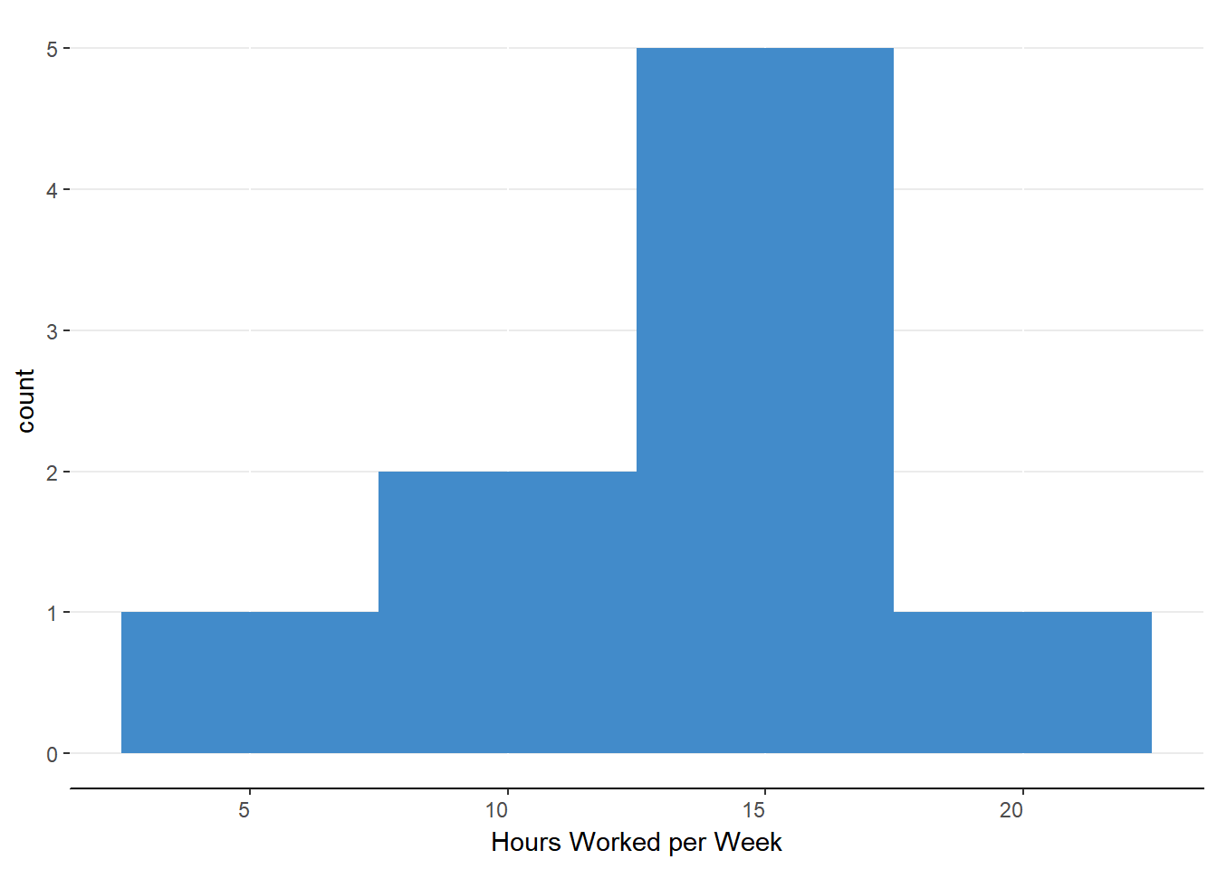
Figure 9.1. Histogram of sample means.
Notice how the peak of the distribution lines up with the population mean. If we investigate this further, we find that the mean of sample means is equal to the population mean
\[ \begin{aligned} M_M&=E(M)=\mu=\frac{\sum{M}}{N_M} \\ &=\frac{20+16.5+13.5+...+10+7}{9} \\ &=\frac{120}{9} \\ &=13.33\text{ hours}\end{aligned} \]
Unbiased Estimator of Population Mean
This is excellent news! The mean of the sampling distribution of sample means is the population mean! The only thing we have to do is determine the mean of every possible sample (of the same size) that can be derived from a population. Actually, that sounds really difficult if not impossible. Even if we had a modest sized population of N = 1,000 individuals and we were to find all of the possible permutations from a group size of 100, we would need to calculate \(N^n = 1000^{100}=1\times10^{300}\). Yes, that means 1 followed by 300 zeros. Worse yet and highly likely, we might not even know the exact size of our population of interest!
What are we to do? Surely we cannot hold off decision making about a population parameter until we exhaust all possible samples. The good news is that we don’t have to wait or even collect multiple samples (although this is a good idea as we’ll discuss in a moment). Because the sample means, on average, equal the population mean, any one sample mean is an unbiased estimator of the population mean.
unbiased estimators are sample statistics (e.g., sample mean) that do not systematically overestimate or underestimate the population parameter. On average, the sample statistics will equal the population parameter.
That is, any given sample mean is equally likely to be an overestimate or underestimate. Of course, we have know way of knowing for sure if our sample mean is greater than or less than the population mean so we assume it to be right in the middle. With any assumption comes error so we will have to incorporate a measure of uncertainty or variability.
Standard Error of the Mean
The sampling distribution of sample means is a normal distribution. As such, it has the typical parameters for normal distributions. We’ve just discussed the mean of sampling distribution of sample means (whoa, what a mouthful) as being equivalent to the population mean. The standard deviation of the sampling distribution of sample means is the standard error of the mean (SEM or \(\sigma_M\)). We calculate the standard error of the mean in the same way that we calculate the standard deviation for a sample. The only differences are that (1) we use the sample means rather than the raw scores and (2) we divide by Nn rather than by n-1. The formula is:
\[ \sigma_M = \sqrt{\frac{\sum(M-\mu_M)^2}{N^n}} \]
Let’s calculate the standard error of the mean for our current example using the table approach.
Table 9.6
Calculating Standard Error of the Mean
| M | M - \(\mu\) | (M-\(\mu\))2 |
|---|---|---|
| 20 | \(20-13.33 = 7.67\) | \(6.67^2 = 44.49\) |
| 16.5 | \(16.5-13.33 = 3.17\) | \(3.17^2 = 10.05\) |
| 13.5 | \(13.5-13.33=0.17\) | \(0.17^2 = 0.03\) |
| 16.5 | \(16.5-13.33 = 3.17\) | \(3.17^2 = 10.05\) |
| 13 | \(13-13.33 = -0.33\) | \(-0.33^2 = 0.11\) |
| 10 | \(10-13.33=-3.33\) | \(-3.33^2 = 11.09\) |
| 13.5 | \(13.5-13.33=0.17\) | \(0.17^2 = 0.03\) |
| 10 | \(10-13.33 =-3.33\) | \(-3.33^2 = 11.09\) |
| 7 | \(7-13.33=-6.33\) | \(-6.33^2 = 40.07\) |
| \(\sum{}=127.01\) |
Now that we have the sum of squares, we divide by the total number of samples (Nn).
\[ \sigma_M^2 = \frac{\sum(M-\mu_M)^2}{N^n}=\frac{127.01}{9}=14.11 \]
The variance of the sampling distribution of sample means is 14.11. To get the standard deviation, we simply take the square root of variance.
\[ \sigma_M = \sqrt{\sigma_M^2}=\sqrt{14.11}=3.76 \]
That means that the sample means are, on average, 3.76 hours of work away from the population mean. The standard error of the mean is, in essence, a measure of sampling error (i.e., how far off might we expect any sample to be). We can decrease this sampling error by increasing our sample size. Conceptually, this means that as we increase our sample size, we are assessing more of the population and thus leaving less room for error.
When you know the population size, the above approach is the most accurate way to determine the standard error of the mean. Unfortunately, we often do not know the population size so we must estimate the standard error of the mean another way. If you have an estimate of the population standard deviation (see below) you can simply divide that by the square root of the sample size.
\[ \sigma_M = \sqrt{\frac{\sigma^2}{n}} = \frac{\sigma}{\sqrt{n}} \]
The Central Limit Theorem
As we’ve discussed several times, normal distributions are very handy for determining probabilities. Unfortunately, some populations are not normally distributed. Do non-normal distributions get left out of statistical analyses and inference? Surely not! Although there are other types of distributions for which statisticians must use for correct inference, we can still utilize sampling distributions of sample means for those non-normal distributions. We can do so because the distribution of sample means collected from a non-normal population tends to be norm. This is particularly true for larger sample sizes (\(n >= 30\)). The interactive figure 9.2 below shows a sampling distribution of sample means based off of a population of 1000 individuals. You can select the sample size on the left to observe how it affects the shape of the sampling distribution of sample means.
Figure 9.2. Central Limit Theorem Interactive Plot
Inferential Statistics
Just as we were able to determine the probability of obtaining a value in a range of z-scores given the mean and standard deviation of some sample, we can extend that procedure to sampling distributions of sample means. That is, we can determine the probability of obtaining some sample mean given a population mean and standard error. Read that last sentence one more time. That sentence is the bridge to hypothesis testing, which will be addressed in the next chapter.
Review of Sampling Distributions of Sample Means
- Sampling distributions of sample means are theoretical distributions. They are not calculated for actual populations. However we can use the proof from small populations to make inferences about larger populations.
- The mean of the sampling distribution of sample means is equal to the population mean.
- The sample mean is an unbiased estimator of the population mean because the sample mean does not systematically overestimate or underestimate the sample mean.
- The standard deviation of the sampling distribution of sample means is called the standard error of the mean. It is a measure of how far, on average, sample means are from the population mean.
- We can use the population mean and the standard error of the mean to determine the probability of obtaining some sample mean.
Sampling Distributions of Sample Variances
Just as we had determined the various samples means for a sampling distribution of sample means, so too can we construct a sailing distribution of sample variances. Let’s build off of the current example data by calculating the variance for each of 9 samples. Recall that variance summarizes how far each value is from the mean, on average.
\[ s^2 = \frac{\sum{(x-M)^2}}{n-1} \]
We’ll discuss why we divide by n-1 rather than n for samples in just a moment. Let’s use the sample variance formula for each sample.
Table 9.7
Calculating Sample Variances
| Sample | Formula | Variance |
|---|---|---|
| A,A | \(\frac{(20-20)^2+(20-20)^2}{2-1}\) | 0 |
| A,B | \(\frac{(20-16.5)^2+(13-16.5)^2}{2-1}\) | 24.5 |
| A,C | \(\frac{(20-13.5)^2+(7-13.5)^2}{2-1}\) | 84.5 |
| B,A | \(\frac{(13-16.5)^2+(20-16.5)^2}{2-1}\) | 24.5 |
| B,B | \(\frac{(13-13)^2+(13-13)^2}{2-1}\) | 0 |
| B,C | \(\frac{(13-10)^2+(7-10)^2}{2-1}\) | 18 |
| C,A | \(\frac{(7-13.5)^2+(20-13.5)^2}{2-1}\) | 84.5 |
| C,B | \(\frac{(7-10)^2+(13-10)^2}{2-1}\) | 18 |
| C,C | \(\frac{(7-7)^2+(7-7)^2}{2-1}\) | 0 |
Unbiased Estimator of Population Variance
How close did any of these samples come to representing the population variance? We typically would not have the population variance for comparison, but because we have the small population information, we can easily calculate the population variance using the following formula:
\[ \begin{aligned} \sigma^2 &= \frac{\sum(x-\mu)^2}{N} \\ &=\frac{(20-13.33)^2+(13-13.33)^2+(7-13.33)^2}{9} \\ &=\frac{44.49+0.11+40.07}{3} \\ &=28.22 \end{aligned} \]
Our population has a variance of \(\sigma^2 = 28.22\) and our samples yielded variances of s2 = 0, s2 = 18, s2 = 24.5 and s2 = 84.5. Once again, none of the generated sample statistics match the population parameter. Perhaps we can better represent the population variance by averaging across our sample variances as we did with the sampling distribution of sample means. Let’s try it out.
\[ \begin{aligned} M_{s^2} &=\frac{0+0+0+18+18+24.5+24.5+84.5+84.5}{9} \\ &= 28.22 \end{aligned} \]
Viola! The mean of the sample variances is the population variance! That is:
\[ M_{s^2} = E(s^2) = \sigma^2 \]
but only when we use n-1 as the denominator for sample variance. If we were to use the full sample size (n) in the denominator, we would underestimate the population variance, on average. When you systematically underestimate or overestimate a population parameter, your estimator is biased. However, our correction of n-1 makes the sample variance an unbiased estimator of the population variance.
There is another important difference with the sampling distribution of sample means. Figure 9.3 is a bar chart of the sample variances. Notice that this is not a normal distribution. In fact, the sampling distributions of sample variances will always be positively skewed.
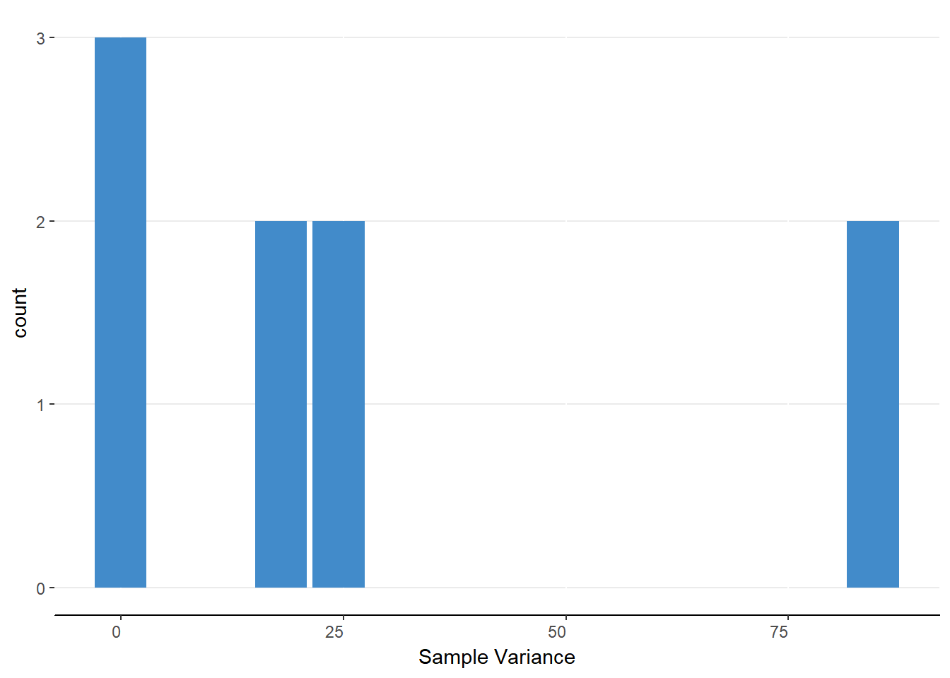
Figure 9.3. Bar chart for calculated sample variances.
Review of Sampling Distributions of Sample Variances
- The unbiased estimator of the population variance (\(\sigma^2\)) is the sample variance s2
- We must use n-1 as the denominator for the sample variance because dividing by n produces an underestimate of the population variance, on average.
- The distribution of sample variances are positively skewed.
Where we are going
Sampling distributions may be tricky to understand at first but it is worth the mental effort up front. Sampling distributions are the basis of the inferences statistics for this course. We will be deciding if an obtained result is statistically significant by comparing that result to an expected sampling distribution. More specifically, we will judging based on the probability of getting some result relative to some expected value. As such, we will need to keep in mind what we’ve learned about probability, the normal distribution, and sampling distributions to be successful for the rest of the course.
Up next is the homework. After you complete and submit the homework, you can complete the quiz.