Data Entry in jamovi
Data Entry in jamoviThe jamovi EnvironmentVariablesEditing a VariableComputeTransformDataSpreadsheetEntering DataEntering Between-Subjects DataEntering Within-Subjects DataAn ExampleSetting Up VariablesEntering Data into the Spreadsheet
The jamovi Environment
jamovi is an free and open-source statistical analysis program based on R. If that doesn't get you excited, perhaps knowing that it is one of the simplest statistical programs to use will pique your interest. jamovi is so simple because it is streamlined and does a great job of producing usable and formatted output. We'll walkthrough each of the parts of the jamovi program before we start adding data.
Variables
The first step in creating a dataset is setting up the structure by creating variables. This happens in the "Variables" tab (see Figure 1)
Figure 1 Variable Tab
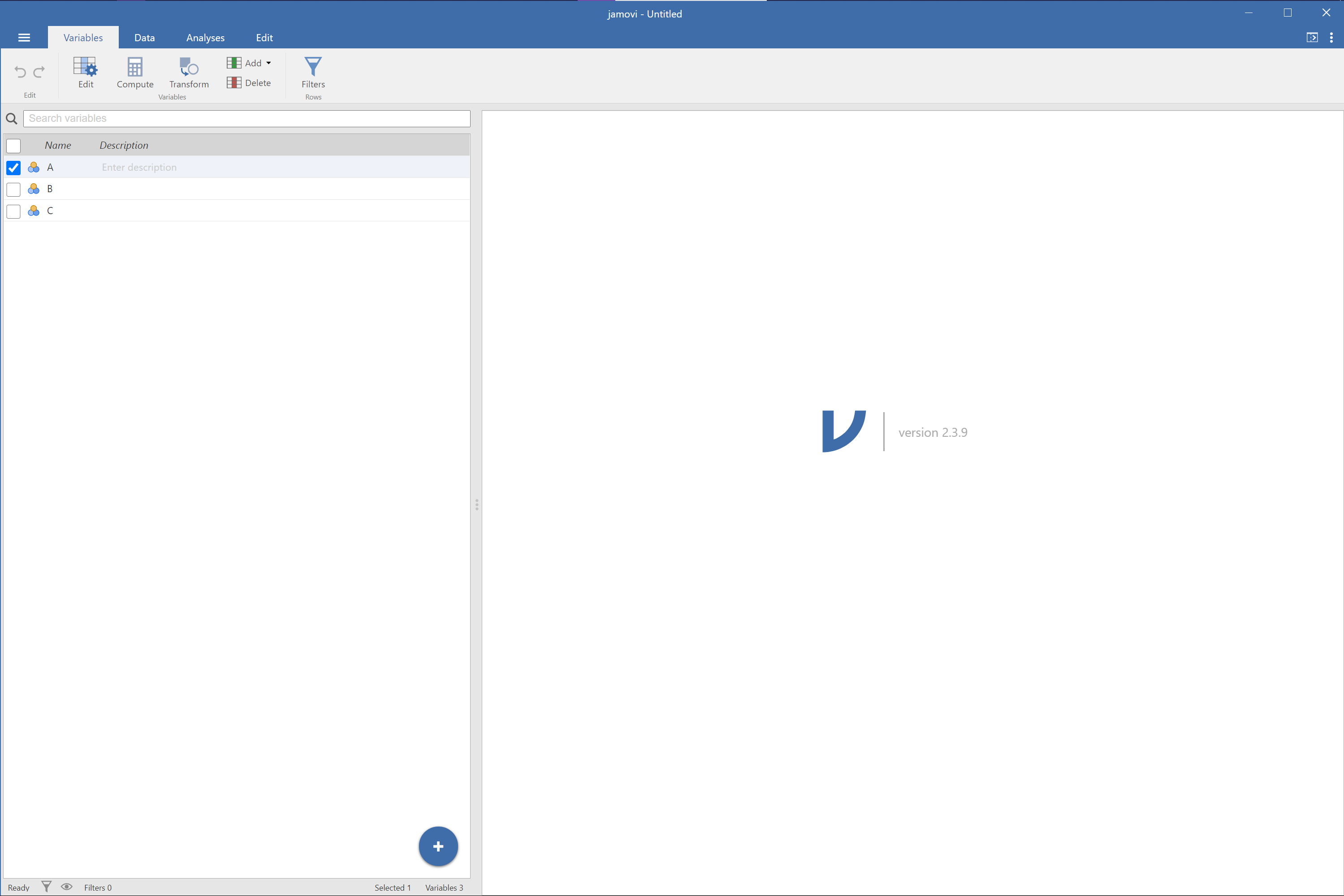
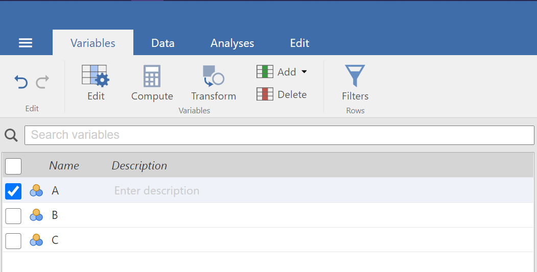
When starting a new file, jamovi defaults to three variables "A", "B", and "C" but you can easily edit, delete, and add variables using the options in the ribbon (see Figure 2)
Figure 2 Variable Tab Ribbon

Editing a Variable
Select a variable by checking the box next to the variable name in the list of variables (see Figure 3).
Figure 3 Selecting a Variable
Click on the "Edit" button  to reveal the variable editing panel (see Figure 4).
Figure 4 Edit Panel
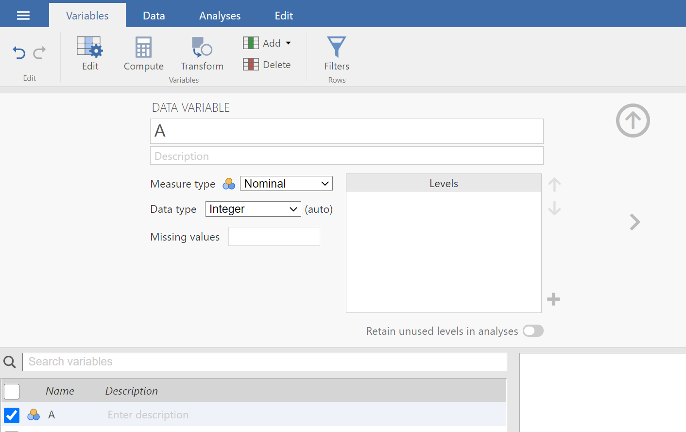
The first field contains the variable name, which can be any combination of characters. I suggest keeping names concise but clear. You can add more details in the "Description" field below the variable name. The "Measure type" field allows you to set the scale of measurement for the variable with the following options: nominal, ordinal, continuous, and ID.
- Nominal: indicates variables with values that differ by kind or type (e.g., genre of music)
- Ordinal: indicates variables with values that can be ordered (e.g., attractiveness)
- Continuous: indicates variables that have values that can be ordered with fixed differences (e.g., age)
- ID: indicates a unique identifier for data that will not be used in analysis (e.g., participant number)
🔎 A Closer Look: Scales of Measurement
The scale of measurement is used to indicate the how much information is included in changes in the values of a variable. Traditionally, there are four scales: nominal, ordinal, interval, and ratio.
Nominal scales indicate a change type or kind but not in amount or rank. For example, hair color or favorite pastime could be considered nominal scale variables because there is not a difference in amount of color between say, red and blonde.
Ordinal scales indicate an ordering of values but not a fixed amount of difference between each value. Placement in a contest is a good example of an ordinal scale. That is, it is clear who was best or fastest when individuals are assigned first, second, or third place. This ranking, however, does not tell you anything about how much better or faster the person in 1st was than the person in 2nd.
Interval scales indicate a fixed and equal increment between values but lacks an "absolute zero." By absolute zero, we are referring to a true absence of whatever is being measured. A fixed and equal increment means that the difference between 10 and 11 is the same as the difference between 15 and 16. The Celsius temperature scale is a good example of this. Although 0 ℃ indicates a freezing temperature for water, it does not indicate an absence of heat and a change from 8 ℃ to 9 ℃ is thought to be the same increase in temperature as the change from 11 ℃ to 12 ℃.
Ratio scales have fixed intervals and and an absolute zero. Scales that involve counting are the best candidates for ratio scales. These include, for example, duration (time), dimensionality (length , volume, etc.), and frequency (occurrences, percentages).
Appropriate Operations
The main reason statisticians are concerned with assigning variables a scale of measurement is that it guides the operations we can perform on those variables. With more information included in the changing of values on the scale, the more complex operations we can perform. Table 1 shows the operations permitted for each scale.
Table 1
Scales and Operations
Scale of Measurement Operations Nominal Count Ordinal Compare, Count Interval Add/Subtract, Compare, Count Ratio Multiply/Divide, Add/Subtract, Compare, Count That is, we can only report how many people have each hair color but cannot say which hair color is "best" (nominal scale). We can report who came in first in the race but cannot say how much faster that person was than the next racer (ordinal scale). We can say how many degrees cooler today is than yesterday but we cannot say how many times hotter yesterday was (interval). We can say how many times larger Jupiter is than the Earth, how many more miles are on Jupiter's equator than the Earth's equator, which has more living inhabitants, and how many colors are reflected by each planet's atmosphere (ratio). This places ratio scale at the top of the order for information-rich scales.
These limiting operations also restrict the summaries we can produce for each scale. Table 2 highlights the measures of central tendency and variability for each scale of measurement.
Table 2
Scales and Summaries
Scale of Measurement Central Tendency Variability Nominal Mode Frequencies Ordinal Median, Mode Interquartile Range (IQR) Interval Mean, Median, Mode Standard Deviation / Variance Ratio Mean, Median, Mode Standard Deviation / Variance These descriptive statistics will be covered in detail in a later chapter but for now, notice how Interval and Ratio scales allow for the same summaries. This is why most statistical programs do not distinguish between them. In jamovi, interval or ratio scales are both classified as "continuous" to reflect their distributions rather than focusing on the presence of absolute zeros.
The next field is the "Data type," which can be set to:
- Integer: any whole number (no decimals)
- Decimal: any dumber with decimals
- Text: any set of letters
Depending on which data type and measure type you select, you may want to enter two or more levels by clicking the plus sign ( + ) to the right of the "Levels" box. Levels are the different possible values of a grouping variable. They can be added to integer data with a nominal or ordinal measure and to text data with a nominal measure.
The last data field is for "Missing values," which tells jamovi when it should not use that for variables. You may want to use missing values as a way to filter out values considered too large or too small or to flag actual missing values during data collection. Clicking on the "Missing values" field will reveal the "MISSING VALUES" panel (see Figure 5).
Figure 5
Missing Values Panel
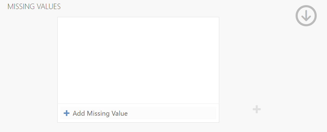
To add missing values, you will need to click on the "+ Add Missing Value" button at the bottom of the list area or the plus (+) button to the right of the list area. This will focus the list area and add the framework code for setting the conditions for when values should be considered missing and thus not used in the analysis (see Figure 6).
Figure 6
Add Missing Value
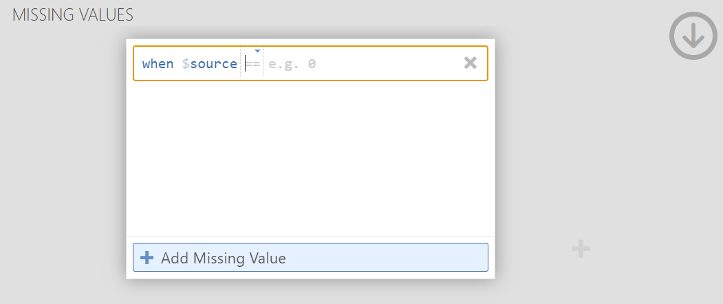
The code is fairly straightforward. When $source is setting up a conditional value for the current variable (i.e., $source). The first area that you'll edit is the conditional operator, for which there are 6 options (see Table 3) presented when you click on the == section.
Table 3
Logical Operator Symbols Meaning
| Symbol | Meaning |
|---|---|
| == | Equal to |
| != | Not equal to |
| > | Greater than |
| < | Less than |
| >= | Greater than or equal to |
| <= | Less than or equal to |
To set one value as a missing value, use == and then type the value you want to consider missing. This value needs to be a possible value for your variable. If you have an integer data type, then you should have an integer (i.e., whole number) as a missing value; if you have text data, then you should have a string (denoted by the single quote marks) as a missing value. When you are done inserting your missing value code, click outside of the highlighted area or press "Enter." You can add as many missing value conditions as you'd like by simply clicking the "+ Add Missing Value" or plus (+) buttons.
📄 Example Code
Missing Value Code for Integer Data
when $source == 9Missing Value Code for Text Data
when $source == 'missed'
Compute
In addition to the "DATA VARIABLE" we reviewed in the last section, we can also determine the values by "computing" them using values from other variables or by "transforming" the all values of an existing variable. Let's check out the "Compute" panel first by clicking on the compute button  , which will open the "COMPUTED VARIABLE" panel (see Figure 7).
Figure 7
Computed Variable Panel
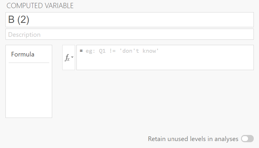
This panel has fewer input fields than the "Edit" options but much can be done in the formula box. You can calculate the average of several variables for each participant, the sum variable values for each participant, or you can calculate an interaction by multiplying two variables together. A few other neat features of computed variables include calculating values for and entire variable and calculations based on groups. Essentially, this will allow you to assign a calculated to each member based on their grouping. We'll get into specific use cases for computed variables in later chapters.
📄 Example Code
= Age * GenderThis will calculate the interaction term for each participant's age and gender
= VMEAN(Age, group_by=Gender)This will assign each participant the mean age for their gender
Transform
Transform offers a more robust way to recode or manipulate existing variables than when using "Compute." To transform a variable, select the existing variable from the variable list then click the "Transform" button  , which reveals the "TRANSFORMED VARIABLE" panel (see Figure 8).
Figure 8
Transformed Variable Panel
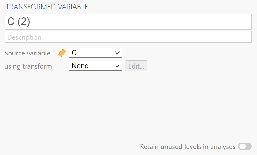
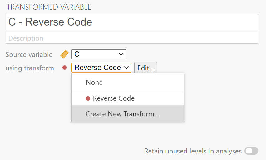
You should rename your variable by updating the text in the first box. I also suggest adding a description in the box directly below the name field. Although you selected a variable before clicking the "Transform" button, you can change which variable you want to transform by selecting from the available variables in the "source variable" dropdown list. The real power of the transform functionality is found in the "using transform" dropdown list. If you've already set up some transformations, they will be listed here, other wise, you'll need to click the "+ Create New Transform" option (see Figure 9). For now, we will enter our variables and data exactly as we want them and we will revisit these transformations in a future chapter.
Figure 9
Transform Dropdown List
Data
With the basics of creating variables complete, we will turn our attention to entering the data. To access the values or enter the values for the variables, click on the "Data" tab at the top of the window this will reveal a new ribbon (see Figure 10).
Figure 10
Data Ribbon

Hopefully most of the options seem familiar as they are the same as those in the "Variables" tab. This is just for convenience. Briefly, I want to mention the last few items in the ribbon before we check out the spreadsheet where data live in jamovi. You can add or delete variables using the "Add" and "Delete" buttons to the right of the "Transform" button. The "Filters" button  reveals the "Row Filters" panel (see Figure 11), where you can tell jamovi which data you want to work with. Importantly, you can save these filters and apply multiple filters simultaneously.
Figure 11
Row Filters Panel
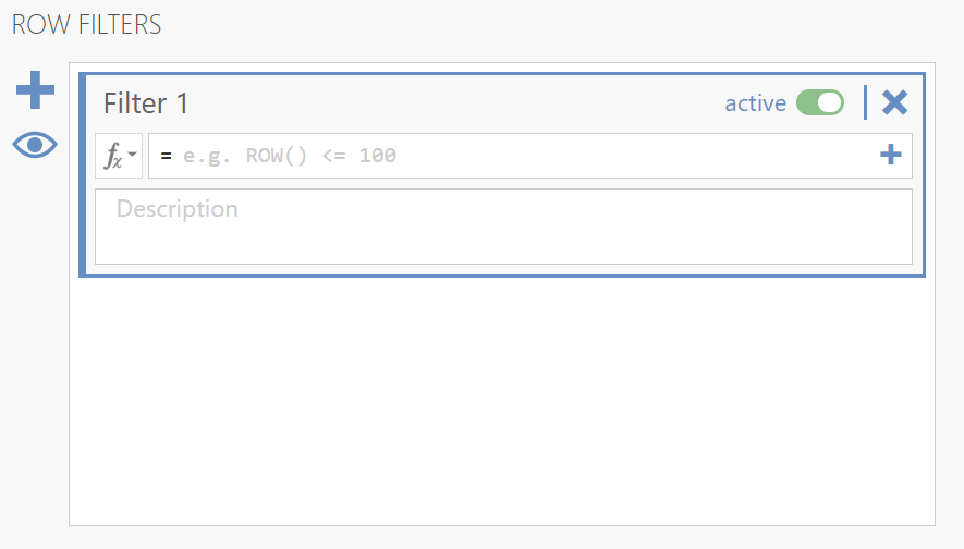
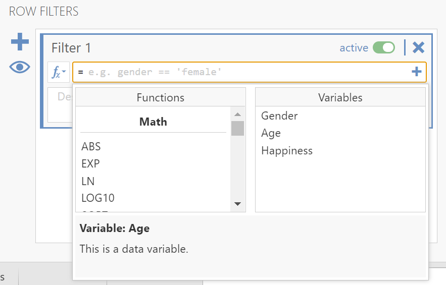
To filter your data, you have to set up a condition much like you do with setting missing values. For example Age > 17 would select all rows in which the participants' age is greater than 17. If you need help building your filter, you can click on the x dropdown to see available functions and variables (see Figure 12).
Figure 12
Function Builder
The last buttons in the ribbon that need addressing are the "Add" and "Delete" rows buttons  . The "Add" options include "Insert," which will add rows above the currently selected row in the spreadsheet, and "Append", which will add rows to the bottom of the spreadsheet. Speaking of the spreadsheet, let's see where the data live.
Spreadsheet
The spreadsheet is so named because it looks like the body of Microsoft's Excel or Google's Sheets. Figure 13 shows a spreadsheet with three variables (columns) and one set of values (row).
Figure 13
The Spreadsheet
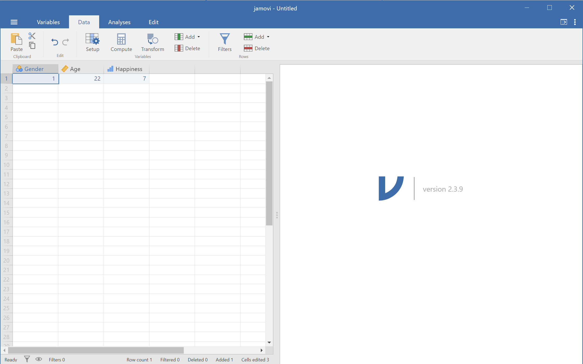
The structure of the spreadsheet is very simple. The columns are the variables you set up under the "Variables" tab but you can also add/delete variables from the ribbon. The rows are linked values for the variables. Values in rows are linked by the entity from which the data are gathered. In psychology, this is typically a person but it could be a business, a school, a country, etc. You may have multiple rows that are connected as you may have multiple values collected per entity. We call these "within-subjects" variables. The "Closer Look" box below compares between- and within-subjects variables.
🔎 A Closer Look: Between-Subjects and Within-Subjects Variables
Between-Subjects Variables are variables in which the values change across "subjects" or "entities" or (in psychology) people. That is, each "subject" can only have one value for that variable. An example may be "sex at birth" or "country of origin" as only one value can be valid for each person.
Within-Subjects Variables are variables in which the values change within "subjects." This means that each entity can have multiple values. This typically occurs with nested designs (e.g., State > county > school district > school) and with longitudinal designs (i.e., measurements taken at different ages).
Entering Data
Entering data in the spreadsheet is very easy. To insert or edit a value, you click in the cell and type the number or text you want to record. You can add new rows simply by clicking in the next blank cell at the bottom of your data or by clicking on the "Add" rows button  . If you want to delete data, you can either use the backspace key while editing the cell or pressing the delete key when the cell is selected. If you want to delete rows, you can select one or multiple rows (i.e., by using
 CTL + clicking on the number starting each row you wish to delete) then pressing the "Delete" rows button  .
.
⚠ CAUTION AHEAD ⚠
A word of caution, jamovi will update the variable properties as you enter your data. This can be helpful when you are entering data before setting up variables (PLEASE DO NOT DO THIS) but is typically unhelpful when you have a mistype. For example, if you have set up a continuous measure variable set to integer data but accidentally hit the "e" key instead of the "3" key, jamovi will change your variable to a nominal measure variable with text data. If this happens, you will need to click the "Setup" button in the data ribbon to reveal the "DATA VARIABLE" panel (or go back to the "Variables" tab) to change the properties.
If you want to add a new variable, you can do so through the "Variables" tab or by clicking the "Add" variable button  . Similarly, you can delete variables by clicking the "Delete" variable button
  or using the "Variables" tab.
Entering Between-Subjects Data
Entering between-subjects data is the easiest because you simply add one row per organizational unit (e.g., "participant"). That is, each person will have one row's worth of data with just one value for each variable.
Entering Within-Subjects Data
Entering within-subjects data is a little more difficult because it requires an "ID" variable and to repeat the values of the between-subjects data across multiple rows. You will need as many rows as you have within-subjects values for each organizational unit. The values for the other variables will be repeated across these rows (including the ID variable).
An Example
Let's walk through a full example of creating a data set by creating the variables, then entering the data. Here is the vignette for this example.
📖 Data Vignette
An emotions researcher is studying how happiness changes across the childhood and across gender. She asks participants to rate their happiness on a scale from 1 ("Very Unhappy") to 10 ("Extremely Happy") when participants are 5, 10, 15, and 20 years old. Below is a table of the data she collected for five participants
Table 1
Happiness Ratings Across Early Life and Gender
Gender 5 years 10 Years 15 Years 20 Years Male 7 8 6 7 Female 4 6 8 9 Male 5 5 5 6 Female 8 6 4 4 Female 6 8 10 9
This vignette has three variables: Gender, Age, and Happiness Rating. Gender is a between-subjects predictor variable as each participant only has one value, Age is a within-subjects variable because each person has four levels/values. Happiness, the outcome variable, which may be referred to as a "repeated measure" because it is assessed repeatedly in the design.
🔎 A Closer Look: Predictors and Outcomes
We have already used several terms to describe our variables (e.g., continuous vs. ordinal vs. nominal, integer vs. decimal vs. text, between- vs. within-subjects). Another dimension on which we can classify variables is the role the variable plays.
Predictor variables are those that are used in a statistical model to estimate the value of another variable. That is, if we know the value of certain predictor variables in our model and the relationships among the variables, we can determine a guess for the value of other variables.
Outcome variables are those that are trying to determine based on our knowledge of how they are related to predictor variables.
Repeated Measures are variables that are assessed multiple times per organizational unit. That is, repeated measures can describe the outcome variable following changes to a within-subjects variable
A business may be interested in estimating how productive (outcome) a potential candidate may be based on factors that can easily be observed or captured in the application and interview (predictors) such as: work history length, positivity of references, personality, etc.
Setting Up Variables
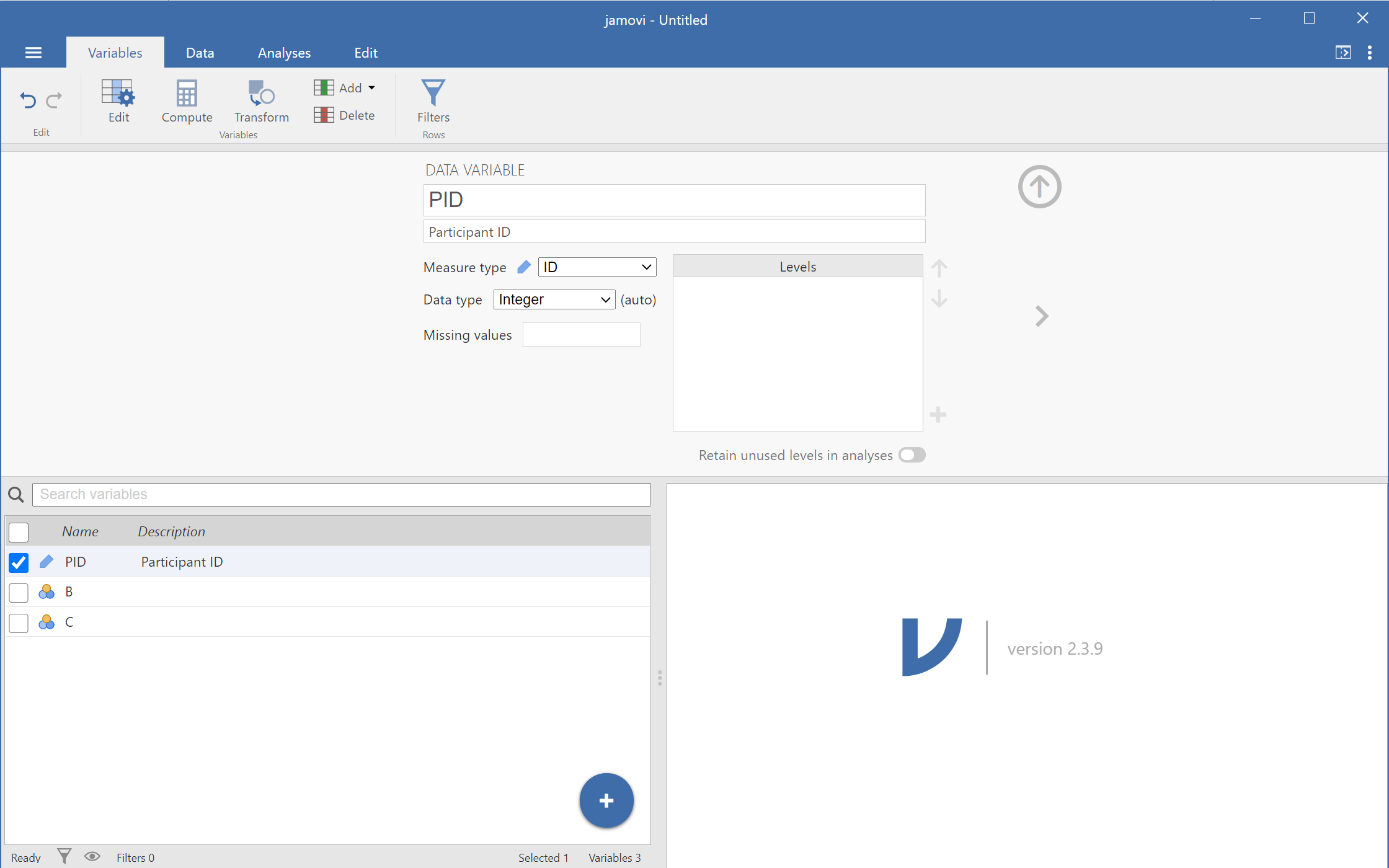
When you start a new jamovi file, you'll get three nominal measure, integer data variables named "A", "B", and "C". We'll use those as our starting point. Click on the "Variables" to find that variable "A" is already selected. Click the "Edit" button  and change the following properties (see Figure 14):
- Name = "PID"
- Description = "Participant ID"
- Measure type = "ID"
- Data type = "Integer"
Figure 14
Editing Variable A
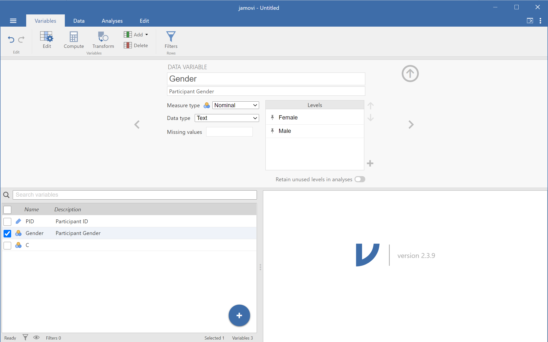
We'll update variable "B" as "Gender" using the following property values (see Figure 15)
- Name = "Gender"
- Description = "Participant Gender"
- Measure type = "Nominal"
- Data type = "Text"
- Levels = "Female", "Male"
Figure 15
Editing Variable B
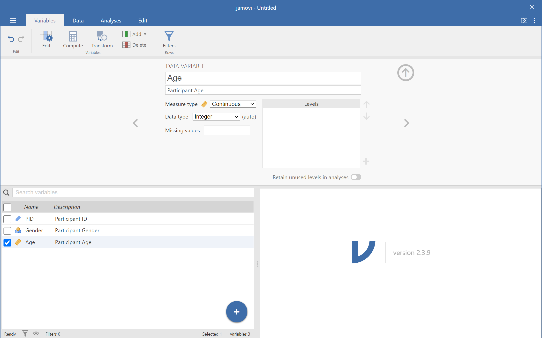
Variable "C" will become "Age" by setting the following properties (see Figure 16)
- Name = "Age"
- Description = "Participant Age"
- Measure type = "Continuous"
- Data type = "Integer"
Figure 16
Editing Variable C
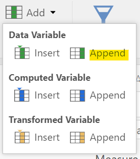
Lastly, we'll need to create a new variable for our "Happiness" scores. Do this by clicking the "Add" variable button  then choosing "Append" the "Data Variable" area (see Figure 17).
Figure 17
Append Data Variable
Set the properties for this new variable ("D") using the following values (see Figure 18)
- Name = "Happiness"
- Description = "Participant Happiness Rating (1 to 10)"
- Measure type = "Ordinal"
- Data type = "Integer"
Figure 18
Editing Variable B
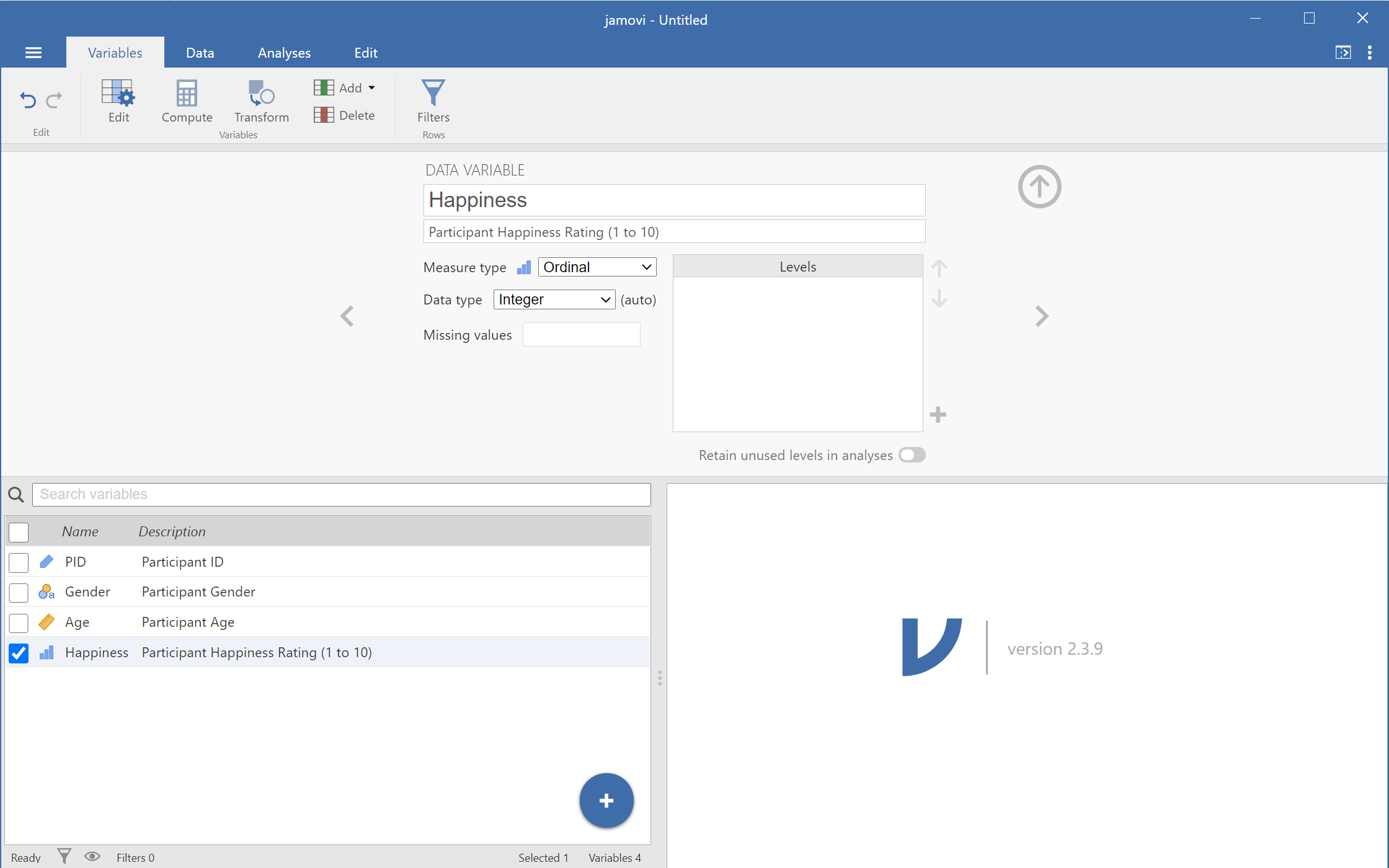
With all of our variables set up, we can now enter our data into the spreadsheet.
Entering Data into the Spreadsheet
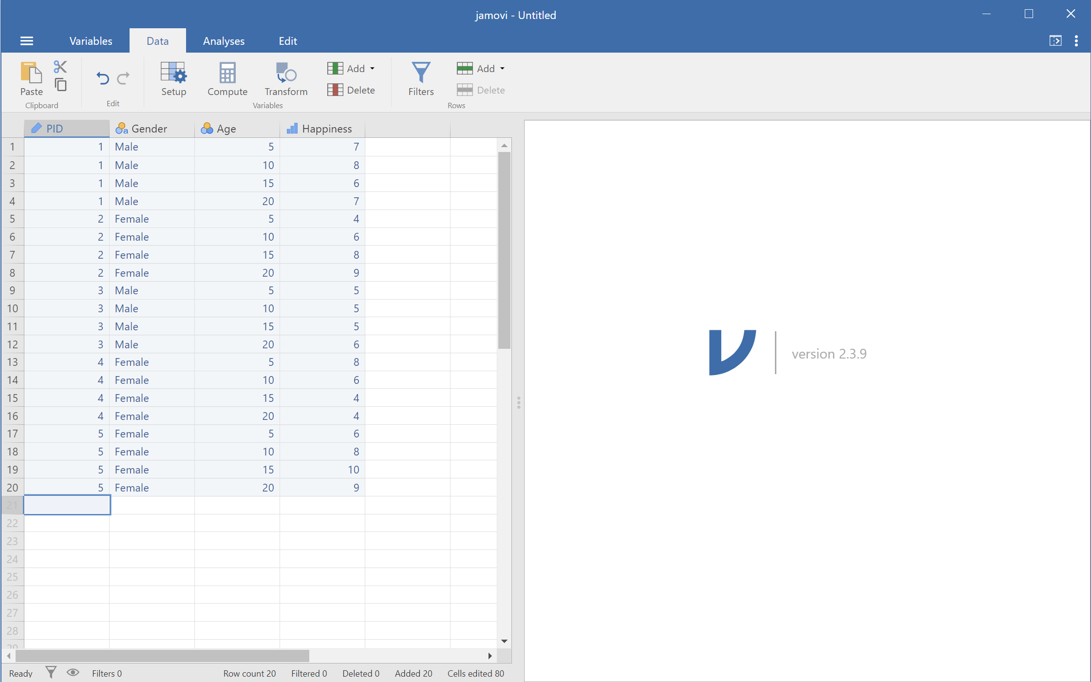
Click on the "Data" tab to see the spreadsheet; there should be no data currently entered. We'll want to ensure we have accurately reproduced the table from our vignette so we need to follow a consistent plan of transferring the data. I recommend entering the "Happiness" values first, then adding in the other predictor variables. Notice that in the table, the happiness ratings for each participant are organized in rows (wide format) but in jamovi, the happiness ratings will be in just one column ("Happiness"). Figure 19 has the happiness ratings for participant 1 entered into the spreadsheet, ordered by Age (ascending).
Figure 19
First Five Happiness Ratings
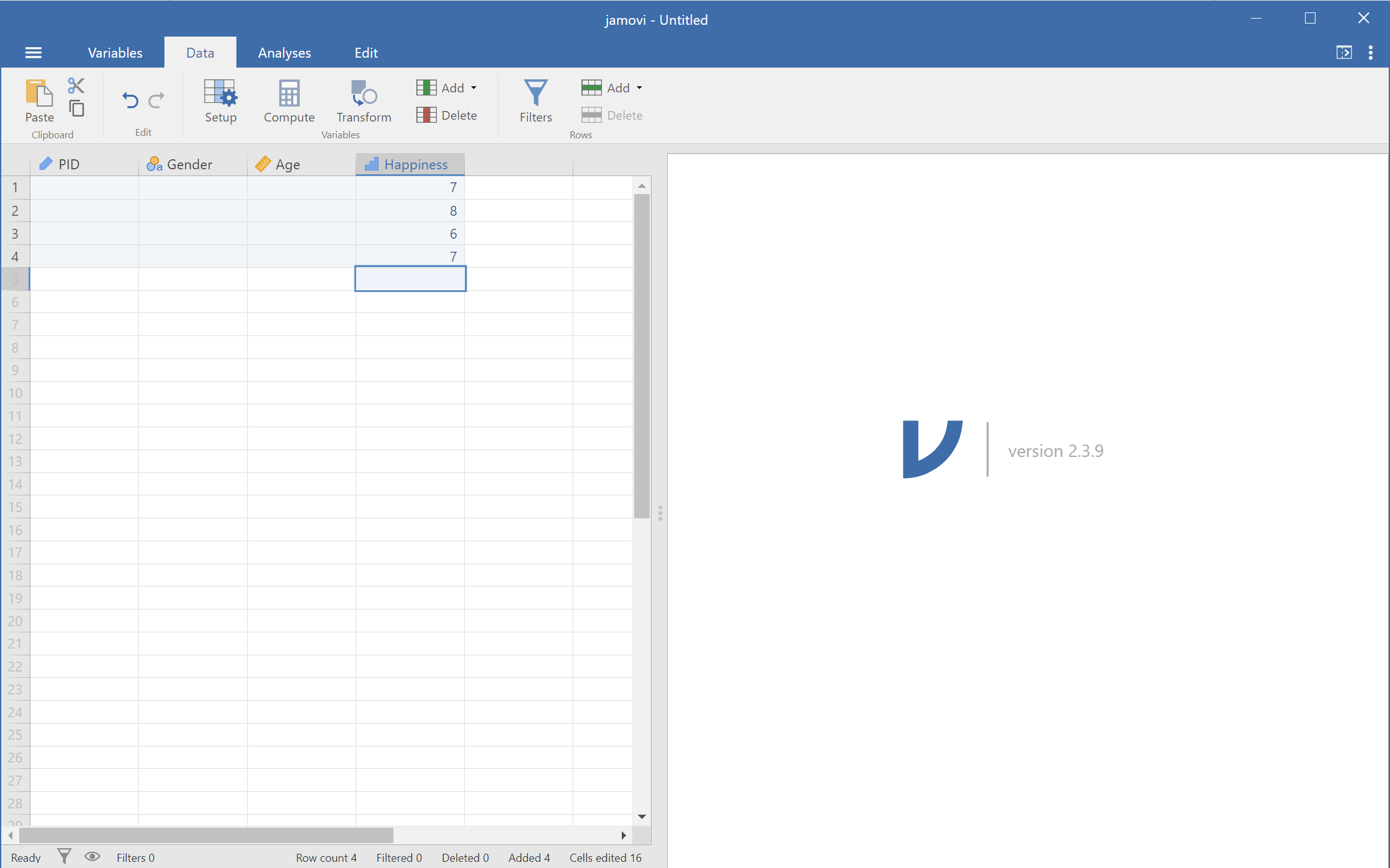
After entering the rest of the happiness ratings, your spreadsheet should look like Figure 20
Figure 20
Complete Happiness Ratings
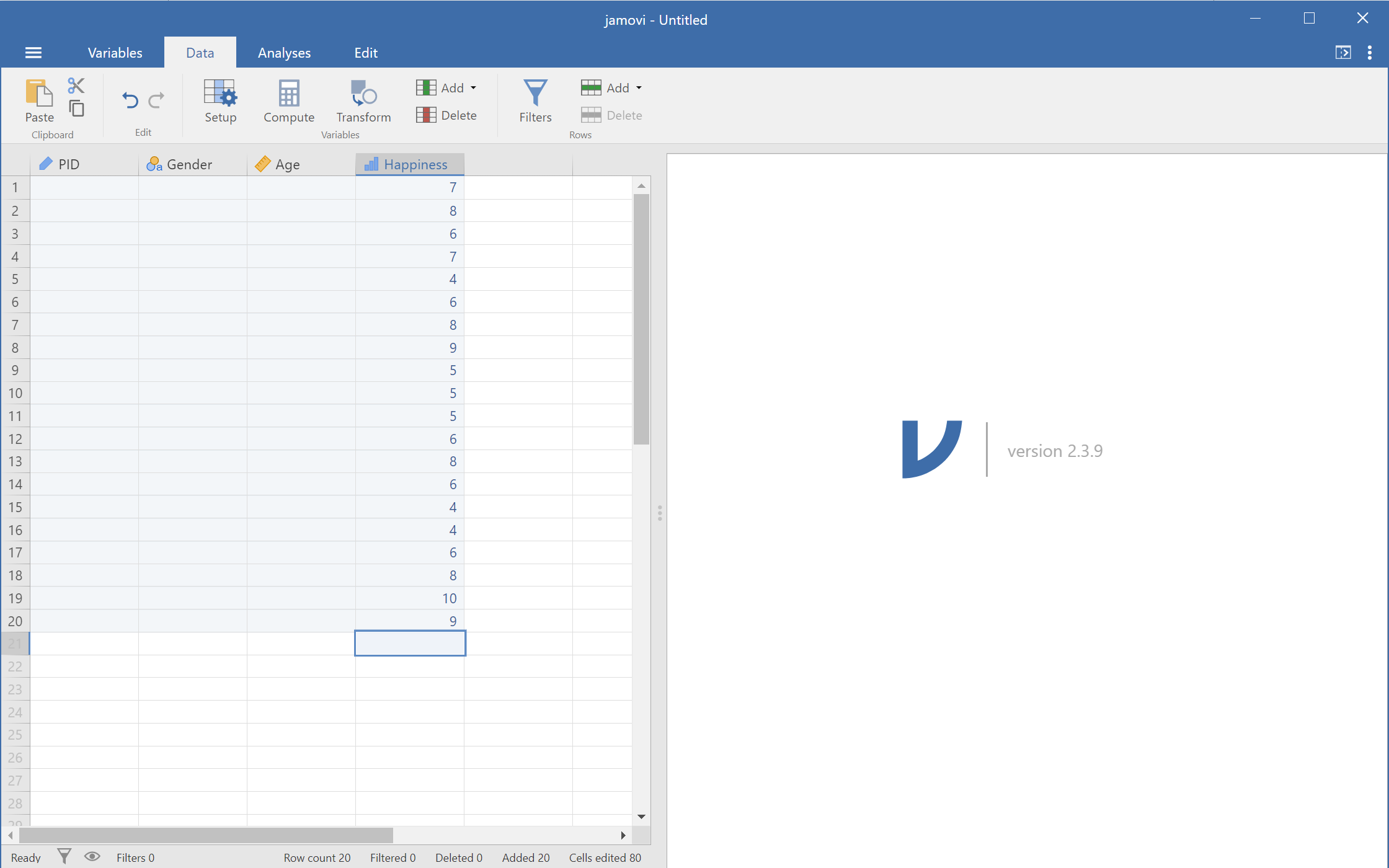
With our repeated-measures outcome variable input complete, let's move to our within-subjects predictor variable, "Age". We can make quick work of this with copy-and-paste because each participant has the same four values (i.e., 5, 10, 15, 20 years). Enter "5" in the first cell below the "Age" header, then follow with "10", "15", "20" (see Figure 21).
Figure 21
First Within-Subjects Values

Now select those four values by clicking and dragging from the first value ("5") to the last ("20") or by clicking on the first value, holding the shift key, and clicking on the last value. To copy those values, press CTL + C on Windows/Linux/Chromebook and ⌘ + C on Mac. Click on the next open cell in the "Age" column and paste the copied values by pressing CTL + V or ⌘ + V (see Figure 22).
Figure 22
Pasting Values in the Spreadsheet
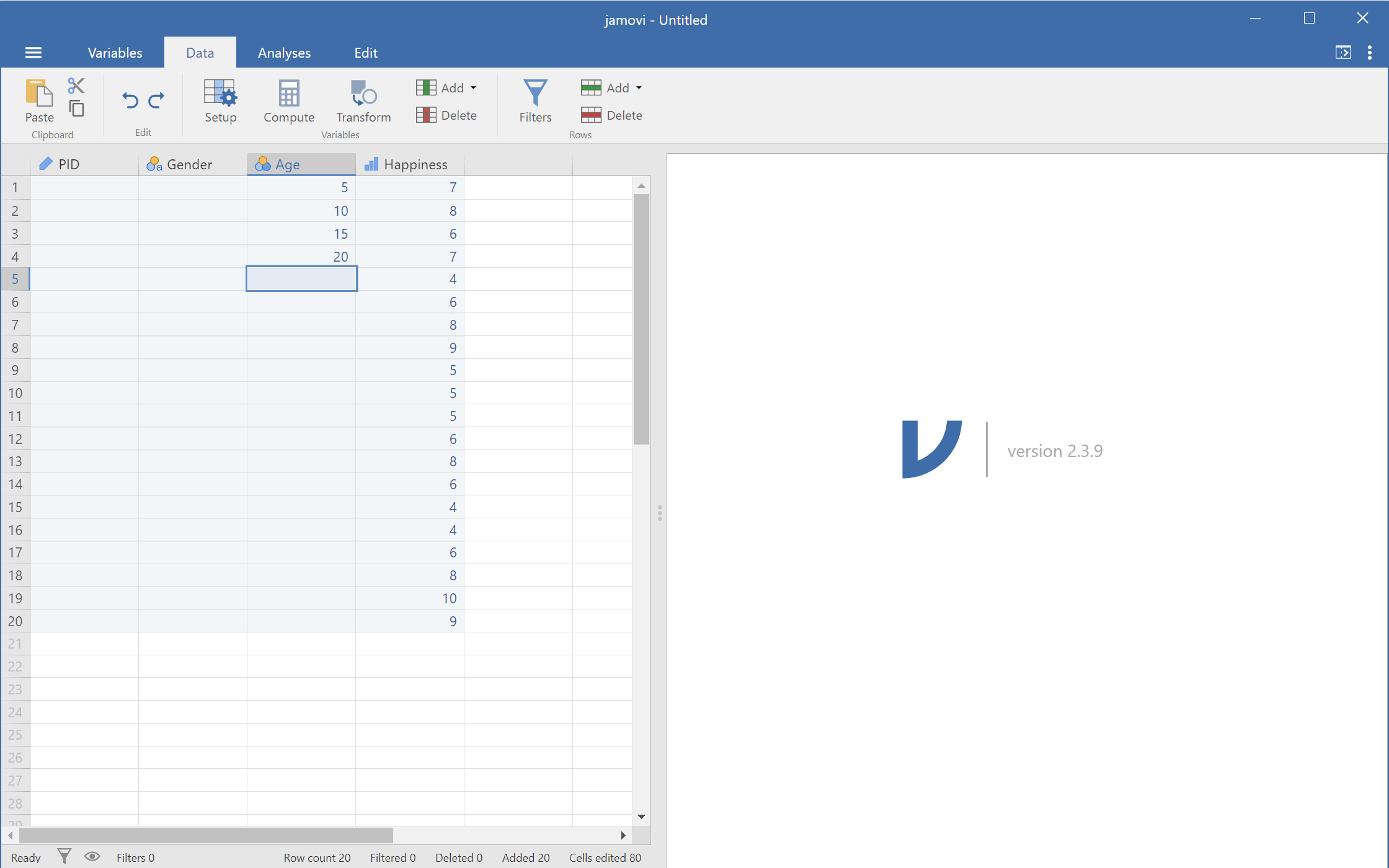
The complete entry for the ages are displayed in Figure 23.
Figure 23
Complete Age Entry
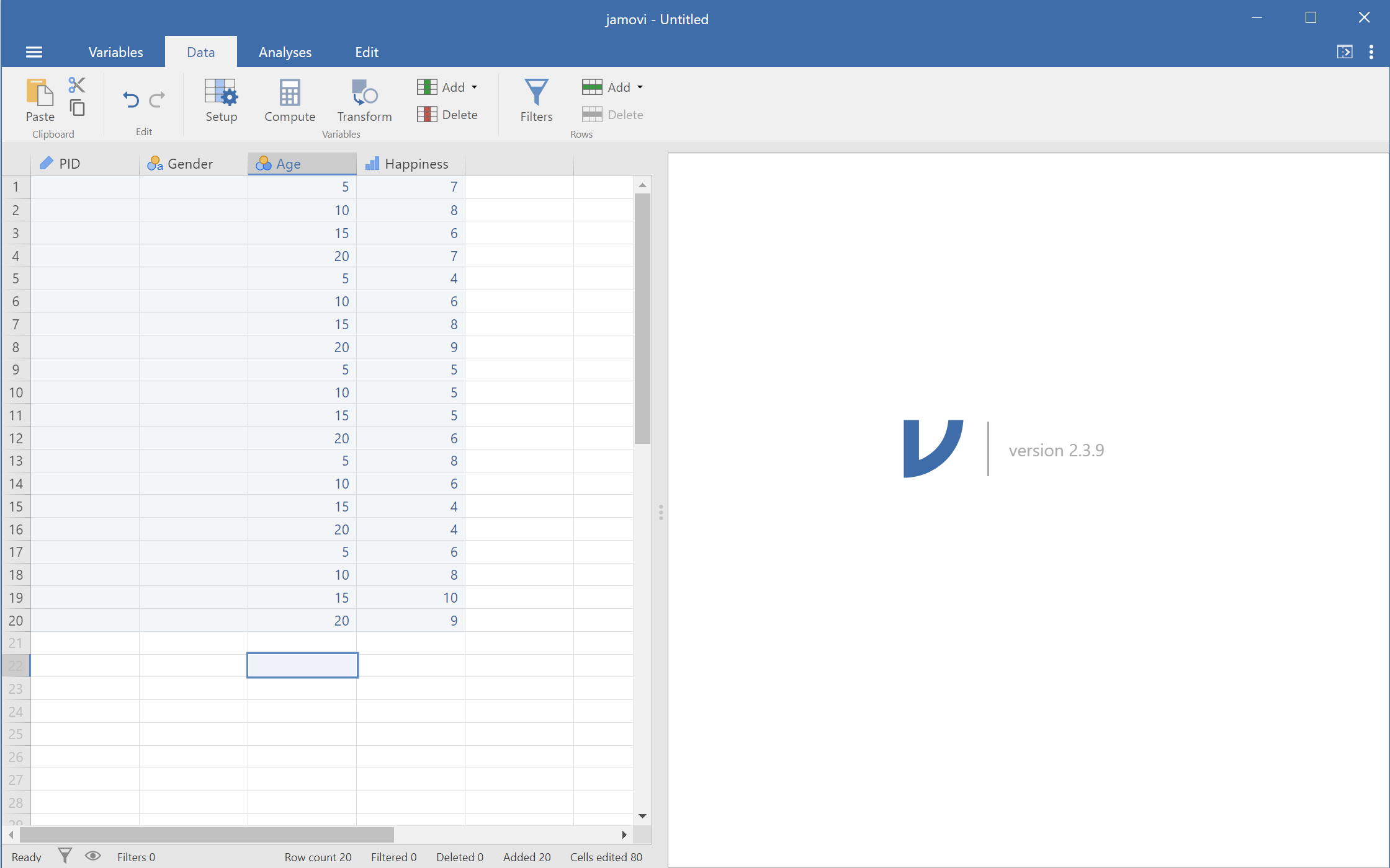
For "Gender", we'll need to make sure that the participant's gender is lined up with their happiness ratings. As you can see in Figure 24, I've entered the participant's gender next to the first age for that participant.
Figure 24
First Gender Entries
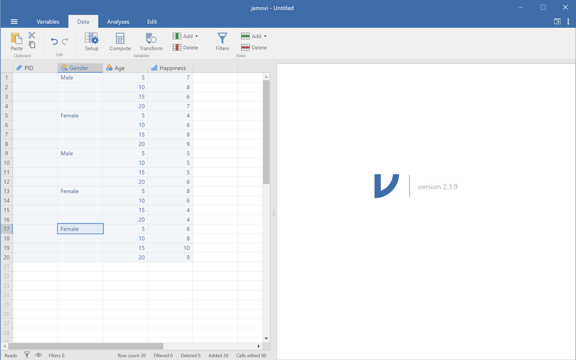
To complete the "Gender" data entry, copy-and-paste to fill in the missing values or you can just type in the values. The completed values for "Gender" are presented in Figure 25.
Figure 25
Completed Gender Entry
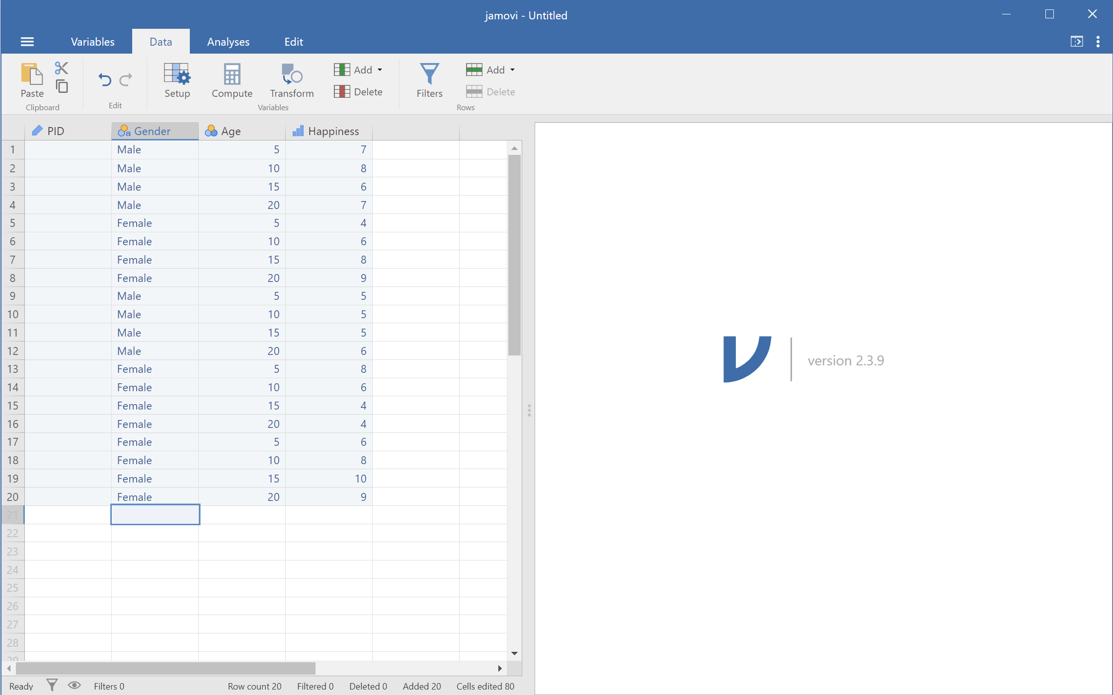
Lastly, we have to complete the "PID" variable. Just like "Gender", each participant will have one value, repeated across all the rows associated with their "Happiness" ratings. I followed the same technique as we did for "Gender" by putting each unique ID on the first line for each participant then filled in the rest. The complete entries for "PID" are in Figure 26.
Figure 26
Completed PID Entry
