The Factorial Between-Subjects ANOVA
The Factorial Between-Subjects ANOVAThe Factorial ANOVAFactorial DesignsRelevant Research QuestionsAssumptionsNull HypothesesExampleEffectsMain EffectsInteraction EffectsSources of VarianceAnalysis Procedure Check AssumptionsTest Main and Interaction EffectsPost Hoc AnalysesOrder of Post Hoc AnalysisTypes of Post Hoc AnalysesSimple Effects TestPairwise Comparison: Tukey HSDUsing jamovi ANOVA for the Factorial Between-Subjects ANOVAThe Research QuestionChecking AssumptionsNormality of DV for Each GroupHomogeneity of VarianceSetting up the Factorial Between-Subjects ANOVAReviewing the output for the Factorial Between-Subjects ANOVAHomogeneity of Variance CheckANOVA TablePost Hoc TestsThe Write-Up of The Factorial Between-Subjects ANOVA
The Factorial ANOVA
We are now at a point to really appreciate the strength of the ANOVA. In the last lesson (within-subjects ANOVA), we saw how we could partition the variance in DV scores due to the participants. We removed that variance from consideration because we were not interested in the effect of the participant. We can use that same approach, however, for other variables. This is exactly what we do in a “factorial” design; investigate the effects of more than one predictor variable.
A factorial design has multiple predictor variables
Factorial Designs
The world is complex. That is, there are many simultaneously impactful factors at work for any given phenomenon. If want to predict who will do well in college, we may want to know more than a student’s gender. Perhaps we may better predict GPA if we add in employment status. In a factorial design, we measure the dependent variable under the combination of levels from more than one independent or predictor variable.
In this lesson, we’ll be examining the factorial between-sujects ANOVA. As you recall, this implies that each participant recieves only one level of each IV. In a fully balanced design, every participant gets exposed to one level of each IV. In unbalanced design, some participants may not receive the manipulation for all IVs.
In a factorial between-subjects design each participant is exposed to just one level of each independent variable.
Relevant Research Questions
Whenever we are wanting to know the impact of multiple *categorical* predictor variables on a *continuous dependent variable, the factorial ANOVA may a good option.
Assumptions
There are assumptions about the data that must be verified for the conclusions of the factorial between-subjects ANOVA to be valid.
- Normal distribution of DV scores within each combination of IV levels.
This requires that we check the distribution of scores after breaking the participants into groups according to the combination of IV levels. As we’ll see in the example, this means checking for normality in each cell.
- Equal variance of DV scores across the IV combination groups.
This requires us to calculated and compare the variance for each cell.
Null Hypotheses
As with our other ANOVA, our null hypothesis is that there is no impact of the IV on DV. The difference here is that we now have multiple IVs so we will have multiple null hypotheses.
As such, for any given effect we test, we assume that the group means are equal to one another and thus that all samples are derived from the same population.
Let’s work with an example to make the factorial ANOVA a little more concrete.
Example
If you recall from the one-way between-subjects ANOVA lesson, we had an example about the effect of different treatments on strawberry sweetness. In that example, we had one variable (i.e., treatment) that had three levels (i.e., none, sugar water, and MiracleGro). Let’s expand that split plot design by adding another factor that might influence strawberry sweetnes: soil.
Dependent Variable: Sweetness Rating (0 - 10)
Independent Variable 1: Treatment (Water vs. Sugar Water vs. MiracleGro)
Independent Variable 2: Soil (Natural vs. Enriched)
Naming Convention
Let’s take a minute to introduce a new naming convention. An ANOVA with only one independent variable are referred to as a one-way ANOVA. An ANOVA with two independent variables may be referred to as a two-way ANOVA. An ANOVA with four independent variables can be called a four-way ANOVA.
We can be a little more informative in our naming by introducing the number of levels of each IV in the name.
For example, rather than just describing an ANOVA as a two-way ANOVA, we might call it a 3x4 ANOVA. This would tell us that the design have two independent variables. The first IV has three levels and the second IV has four levels.
Here is the breakdown.
*The number of terms tells you the number of independent variables.*
An AxBxCxD ANOVA would have 4 independent variables. An AxB ANOVA would have 2.
*The value of each term tells you the number of levels for that independent variable.*
A 2x4x3 ANOVA has an IV with 2 levels, another IV with 4 levels, and another IV with 3 levels.
Table 1 represents a 3x2 split plot design with our two variables.
Table 1
Representation of Two-Factor Split Plot Design
| Water | Sugar Water | MiracleGro | |
|---|---|---|---|
| Natural | 1 | 0 | 5 |
| 2 | 0 | 6 | |
| 1 | 1 | 7 | |
| Enriched | 2 | 0 | 9 |
| 3 | 1 | 8 | |
| 3 | 1 | 10 |
You may see the similarity with the one-way within-subjects ANOVA at this point in how we have a grouping by rows instead of just by columns. There are some important differences, however. We now have more than one effect we’ll want to test.
Effects
In factorial designs, we will have two kinds of effects: main effects and interaction effects.
Main Effects
We are familiar with main effects as they are similar to what we tested in the one-way ANOVAs. A main effect is the impact of changing the levels of just one IV on the DV. That means that a main effect will only consider the impact of one IV at a time on the DV. You will have one main effect to test for each IV.
Main effects are the impact of one IV on the DV, regardless of the other IVs.
In our example, we would test for main effect of treatment and a main effect of soil.
The main effects are a comparison of the marginal means for each IV to the grand mean. Table 2 includes the marginal means for both treatment and soil.
Table 2
Marginal Means for Main Effects
Table 1
Representation of Two-Factor Split Plot Design
| Water | Sugar Water | MiracleGro | Marginal Mean (Soil) | |
|---|---|---|---|---|
| Natural | 1 | 0 | 5 | |
| 2 | 0 | 6 | 2.56 | |
| 1 | 1 | 7 | ||
| Enriched | 2 | 0 | 9 | |
| 3 | 1 | 8 | 4 | |
| 3 | 1 | 10 | ||
| Marginal Mean (Treatment) | 2 | 0.5 | 7.33 | GM = 3.28 |
Interaction Effects
Although it is convenient to test two variables in the same sample, the more imporant benefit of the factorial ANOVA is the ability to test for an interaction effect of two or more variable. You may have heard of interaction effects in relation to medications. Usually, you hear about the negative side effects that can occur when combining medications. The key point is that either may be a safe drug when taken alone but when the drugs are acting simultaneously, a new effect emerges. As such, interaction effects are the changes that occur in the dependent variable because of the combination of multiple independent variables.
Interaction effects are the combined impact of IVs on the DV.
There are two types of interaction effects. The first is called a crossover interaction because the pattern of the means changes directions as the other IV changes levels. Figure 1 demonstrates the crossover interaction
Figure 1
Crossover Interaction

The other type of interaction is an ordinal interaction. Rather than switching directions, the difference in means across the levels in one IV increases or decreases as the levels of the other IV change. Figure 2 represents an ordinal interaction.
Figure 2
Ordinal Interaction

In both cases, we can judge if an interaction effect is likely by the divergence of our lines from parallel.
In our example, we would test for one interaction effect, the treatment x soil (read as “treatment by soil”) interaction. This effect is tested by comparing the cell means (i.e., the mean sweetness of strawberries grown with water in natural soil) to the grand mean. Table 3 adds the cell means to the marginal means of Table 2.
Table 3
Cell Means for Interaction Effect
| Water | Sugar Water | MiracleGro | Marginal Mean (Soil) | |
|---|---|---|---|---|
| Natural | 1 | 0 | 5 | |
| 2 | 0 | 6 | 2.56 | |
| 1 | 1 | 7 | ||
| M = 2 | M = .33 | M = 6 | ||
| Enriched | 2 | 0 | 9 | |
| 3 | 1 | 8 | 4 | |
| 3 | 1 | 10 | ||
| M = 2.67 | M = 0.67 | M = 8 | ||
| Marginal Mean (Treatment) | 2 | 0.5 | 7.33 | GM = 3.28 |
Note. Pink highlighted cells relate to the interaction effect of Soil x Treatment.
Sources of Variance
The ANOVA approach is all about partitioning the variability in the DV scores. We had previously divided the variance into the effect variance and the error variance (we also separated the variance due to participants for the within-subjects design). The factorial ANOVA uses the same approach to partition variance into main effect variance, interaction effect variance, and error variance.
We discussed the sources for the main and interaction effects in the previous section. Where is the error? Remember that the “error” variance is the left over variance in the dependent variable that we cannot account for. The main effects account for variability across rows and columns. The interaction effect accounts for variability across cells. What is left? The variability within cells (i.e., the difference among values and the cell means)! Table 4 highlights the error variance.
Table 4
Within Cell Variance as Error Variance
| Water | Sugar Water | MiracleGro | Marginal Mean (Soil) | |
|---|---|---|---|---|
| Natural | 1 | 0 | 5 | |
| 2 | 0 | 6 | 2.56 | |
| 1 | 1 | 7 | ||
| M = 2 | M = .33 | M = 6 | ||
| Enriched | 2 | 0 | 9 | |
| 3 | 1 | 8 | 4 | |
| 3 | 1 | 10 | ||
| M = 2.67 | M = 0.67 | M = 8 | ||
| Marginal Mean (Treatment) | 2 | 0.5 | 7.33 | GM = 3.28 |
Note. Blue highlighted values relate to the calculation of error variance.
You can all of these sources of variance represented for our example in Table 5 in the next section.
Analysis Procedure
Check Assumptions
The first step in the factorial ANOVA is to verify that the assumptions hold.
You can check the assumption regarding normality by producing histograms or Q-Q plots for each combination of factor levels (see walkthrough below).
You can check the assumption of homogeneity of variance by producing a simple error bar chart and checking Leven’s test for the equality of variances (see walkthrough below).
Test Main and Interaction Effects
The ANOVA procedure in jamovi will produce an ANOVA table.
Table 5 representes an ANOVA table for our example of the impact of soil and treatment on strawberry sweetness
Table 5
ANOVA Table for Sweetness Example
| Source | Sum of Squares | df | Mean Square | F | p | η2p |
|---|---|---|---|---|---|---|
| Treatment | 163.00 | 2 | 81.500 | 146.70 | <.001 | .961 |
| Soil | 10.89 | 1 | 10.899 | 19.60 | <.001 | .620 |
| Treatment x Soil | 5.44 | 2 | 2.722 | 4.90 | .028 | .450 |
| Residuals | 6.67 | 12 | 0.566 | – | – |
As we had done with previous ANOVA, we will check the p column for values less than .05 (our alpha-level). If the p-value s less than .05, we reject the null hypothesis for that effect. We will need to do this for each effect in our table.
In our example, each main effect and the interaction effect are statistically significant. Recall that a significant F-value tells us that there is a difference among means, somewhere, but not which means are reliably different. As such, we will likely need post-hoc analyses to elucidate the pattern of means. This is true EXCEPT FOR IVs WITH ONLY 2 LEVELS. If one of your IVs only has two levels, then you know that the two sample means are reliably different from the ANOVA and you do not need to perform a separate post hoc analysis.
Post Hoc Analyses
Order of Post Hoc Analysis
There are three significant effects (one for treatment, one for soil, and one for the interaction of treatment by soil). Which should we investigate further first?
If you have a significant interaction effect, start with that interaction effect. Interaction effects will tell you the most about how the IVs effect the DV. Furthermore, in some cases, the main effects main contradict the interaction effect. As such, the more nuanced story (i.e., the interaction effect) is the better story to tell.
Order of Post Hoc Analyses
- Significant interactions should be investigated first because they have the most amount of detail regarding how the IVs impact the DV.
- If the interaction is not significant, investigate the significant main effects.
- If no effects are statistically significant, do not perform (or interpret) post hoc analyses.
Types of Post Hoc Analyses
Before we get to how to perform post hoc analyses, let’s revisit why we want to perform post hoc analyses. We want to know about the pattern of means. We want to know how changing the level of IVs impacts the DV scores. This is especially important for the interaction effect.
Simple Effects Test
If we have a statistically significant interaction effect, it is telling us the impact of one IV on the DV changes as we change the levels of the other IV. As such, we may want to examine the effect of one IV within the levels of the other IV. That is, we take the data the was collected under one condition of one IV and test for the effect of the other IV on the DV. This approach is called the simple effects test.
The simple effects test ivnestigates the effect of one IV on the DV within each level of another IV.
In our example, we will test the effect of treatment in the “natural” soil condition and then separately in the “enriched” soil condition using one-way ANOVA. Tables 6 and 7 are the results of the simple effects tests within each type of soil.
Table 6
Simple Effects Test of Treatment within Natural Soil
| Source | Sum of Squares | df | Mean Square | F | p | η2 |
|---|---|---|---|---|---|---|
| Treatment | 54.89 | 2 | 27.44 | 49.40 | <.001 | 0.943 |
| Error | 3.33 | 6 | 0.556 | – | – |
Table 7
Simple Effects Test of Treatment within Enriched Soil
| Source | Sum of Squares | df | Mean Square | F | p | η2 |
|---|---|---|---|---|---|---|
| Treatment | 113.56 | 2 | 56.778 | 102 | <.001 | 0.971 |
| Error | 3.33 | 6 | 0.556 | – | – |
With the effect of treatment being very large and statistically significant in both conditions of soil (Fs > 49, ps < .001), we can move into the next post hoc analysis: pairwise comparisons.
Pairwise Comparison: Tukey HSD
The Tukey HSD is the appropriate analysis for a follow up to the simple effects test because the simple effects test was just a one-way between-subjects ANOVA.
Remember that the Tukey HSD test is preferable to an independent sample t-test because it controls for multiple tests so that we maintain an overall alpha level equal to 0.05. That is, it prevents us from inflating our type I error rate.
Tables 8 and 9 present the results fo the Tukey HSD tests for treatement in the natural and enriched soil conditions, respectively.
Table 8
Tukey HSD Test of Treatment within Natural Soil
| TreatmentA | TreatmentB | Mean Difference | SE | df | t | ptukey | Cohen's d |
|---|---|---|---|---|---|---|---|
| Water | Sugar Water | 1.00 | 0.609 | 6.00 | 1.64 | 0.300 | 1.34 |
| Water | MiracleGro | -4.67 | 0.609 | 6.00 | -7.67 | < .001 | -6.26 |
| Sugar Water | MiracleGro | -5.67 | 0.609 | 6.00 | -9.31 | < .001 | -7.60 |
Table 9
Tukey HSD Test of Treatment within Enriched Soil
| TreatmentA | TreatmentB | Mean Difference | SE | df | t | ptukey | Cohen's d |
|---|---|---|---|---|---|---|---|
| Water | Sugar Water | 2.00 | 0.609 | 6.00 | 3.29 | 0.038 | 2.68 |
| Water | MiracleGro | -6.33 | 0.609 | 6.00 | -10.41 | < .001 | -8.50 |
| Sugar Water | MiracleGro | -8.33 | 0.609 | 6.00 | -13.69 | < .001 | -11.18 |
It seems that we’ve found the important change across soil conditions. Whereas the differences among the treatments are all statistically significant (ps < .05) in the enriched soil condition, the difference between water and sugar was not reliably different in the natural soil condition (p = .300).
Interestingly, Cohen's d is very large for the comparison that is not statistically significant. How can that be? Cohen's d is a characterization of how different the two sample means are (in standard deviations). That is, Cohen's d standardizes the effect of our two levels of treatment on sweetness. The p-value represents the probability of claiming that there is an effect in the population when there is no effect. In our example, we would have 30% chance of making an error. The supplement to this is confidence. We would only have 70% confidence in claiming an effect at the population level. Typically, our chances of making an error go down and our confidence increases as our sample size increases (i.e., incorporating more of the population). So our very large effect in our sample may be an indication of the effect in the population but we cannot, with high confidence, claim that to be the case. The real issue, here, is a lack of statistical power stemming from small sample sizes.
Statistical power is the probability of detecting a true effect. That is, the probability of correctly rejecting the null hypothesis. This is calculated as 1 - β, where β is the probability of maintaining the null hypothesis when the null hypothesis is false.
Power is influenced by α, sample size, and effect size. To increase power, the researcher can:
- Increase α (but this increases type I error rate)
- Increase sample size (n)
Effect size is what is observed and cannot be altered (although it is influenced somewhat by sample size). Generally speaking, the most convincing results are those that report a large effect, large sample size, and a conservative (e.g., small) α.
It can be hard to interpret interaction effects through post hoc analyses alone. An interaction plot can help to reinforce what is expressed in these analyses. Figure 3 represents the interaction between soil and treatment on strawberry sweetness
Figure 3
Interaction Plot of Soil and Treatment on Sweetness
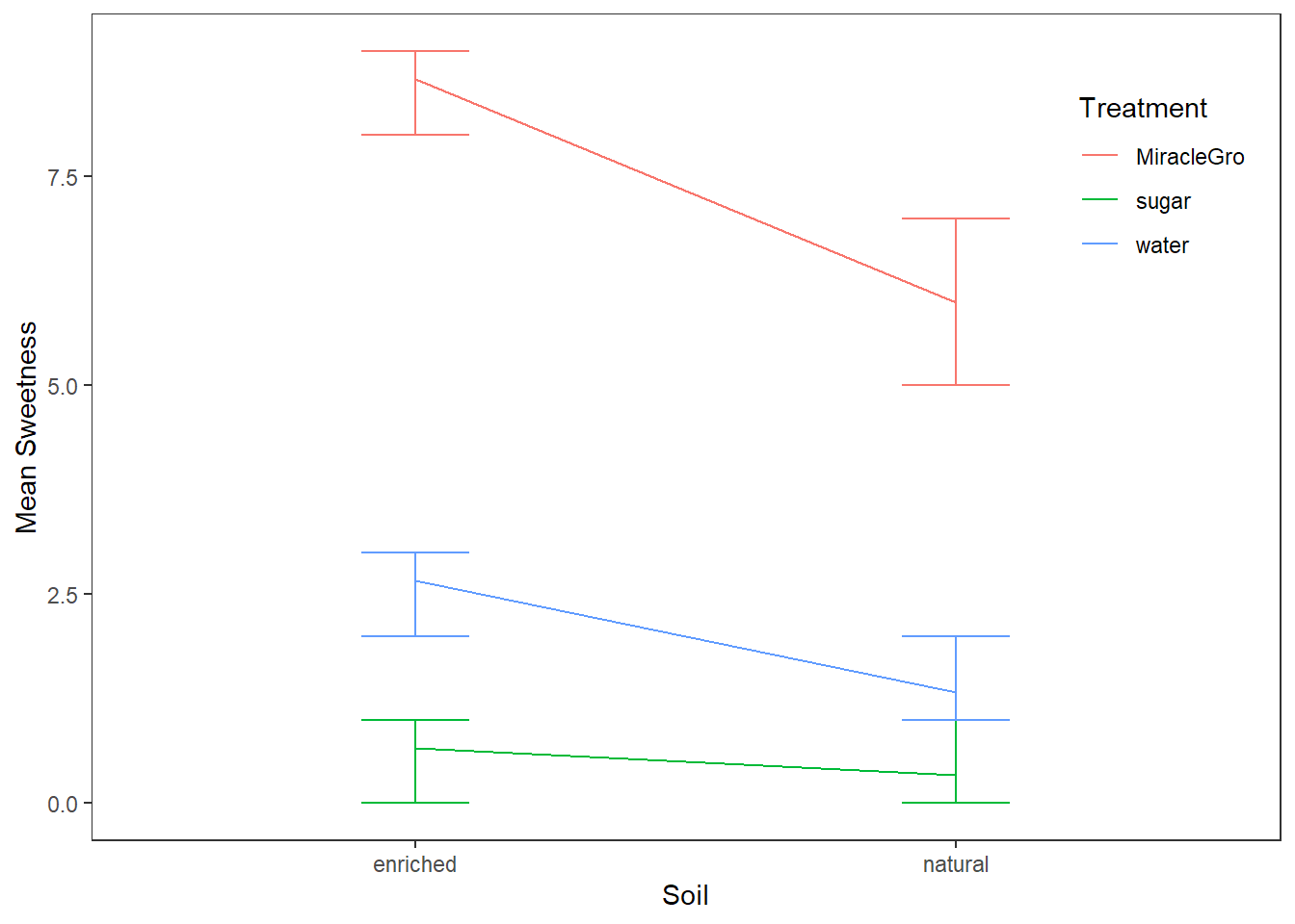
Note. Error bars represent 95% CI.
As we saw across tables 8 and 9, the difference in sweetness for strawberries grown in natural soil were significant for MiracleGro and Sugar or Water but not between Sugar and Water. In contrast, all treatments yielding significantly different sweetness ratings in the enriched soil.
Depending on the guiding hypotheses, you may want to perform your pairwise comparisons differently. Perhaps I am interested in the best overall approach to growing sweet strawberries. That is, perhaps I won’t to directly compare all conditions. If this is the case, we would want to put all combinations of the IVs into a Tukey HSD test. Table 10 presents the results of such a test.
Table 10
Tukey HSD Using All Pairwise Comparisons
| Treatment | Soil | Treatment | Soil | Mean Difference | SE | df | t | ptukey | Cohen's d |
|---|---|---|---|---|---|---|---|---|---|
| Water | Natural | Water | Enriched | -1.333 | 0.609 | 12.0 | -2.191 | 0.309 | -1.789 |
| Sugar Water | Natural | 1.000 | 0.609 | 12.0 | 1.643 | 0.589 | 1.342 | ||
| Sugar Water | Enriched | 0.667 | 0.609 | 12.0 | 1.095 | 0.874 | 0.894 | ||
| MiracleGro | Natural | -4.667 | 0.609 | 12.0 | -7.668 | < .001 | -6.261 | ||
| MiracleGro | Enriched | -7.667 | 0.609 | 12.0 | -12.598 | < .001 | -10.286 | ||
| Enriched | Sugar Water | Natural | 2.333 | 0.609 | 12.0 | 3.834 | 0.022 | -3.130 | |
| Sugar Water | Enriched | 2.000 | 0.609 | 12.0 | 3.286 | 0.056 | 2.683 | ||
| MiracleGro | Natural | -3.333 | 0.609 | 12.0 | -5.477 | 0.002 | 4.472 | ||
| MiracleGro | Enriched | -6.333 | 0.609 | 12.0 | -10.407 | < .001 | -8.497 | ||
| Sugar Water | Natural | Sugar Water | Enriched | -0.333 | 0.609 | 12.0 | -0.548 | 0.993 | -0.447 |
| MiracleGro | Natural | -5.667 | 0.609 | 12.0 | -9.311 | < .001 | -7.603 | ||
| MiracleGro | Enriched | -8.667 | 0.609 | 12.0 | -14.241 | < .001 | -11.628 | ||
| Enriched | MiracleGro | Natural | -5.333 | 0.609 | 12.0 | -8.764 | < .001 | 7.155 | |
| MiracleGro | Enriched | -8.333 | 0.609 | 12.0 | -13.693 | < .001 | -11.180 | ||
| MiracleGro | Natural | MiracleGro | Enriched | -3.000 | 0.609 | 12.0 | -4.930 | 0.004 | -4.025 |
As we expected from Figure 3, apply MiracleGro to strawberry plants in enriched soil lead to reliably sweeter strawberries than any other Soil x Treatment condition. We can tell this because all Tukey HSD post hoc tests involving the MiracleGro in enriched soil were statistically significant.
Using jamovi ANOVA for the Factorial Between-Subjects ANOVA
I will walk you through the full procedure for conducting the factorial between-subjects ANOVA, post-hoc tests, and the write-up using jamovi and the teaching example dataset I've used in the previous posts.
The Research Question
For this example, we will want to determine "how do one's marital status and country of origin impact happiness ratings before mindfulness training?" Because our dataset is in the wide format, we'll choose just one sample of our outcome variable. In this case, I'm using the average happiness ratings that were collected before mindfulness training was completed.
Checking Assumptions
Normality of DV for Each Group
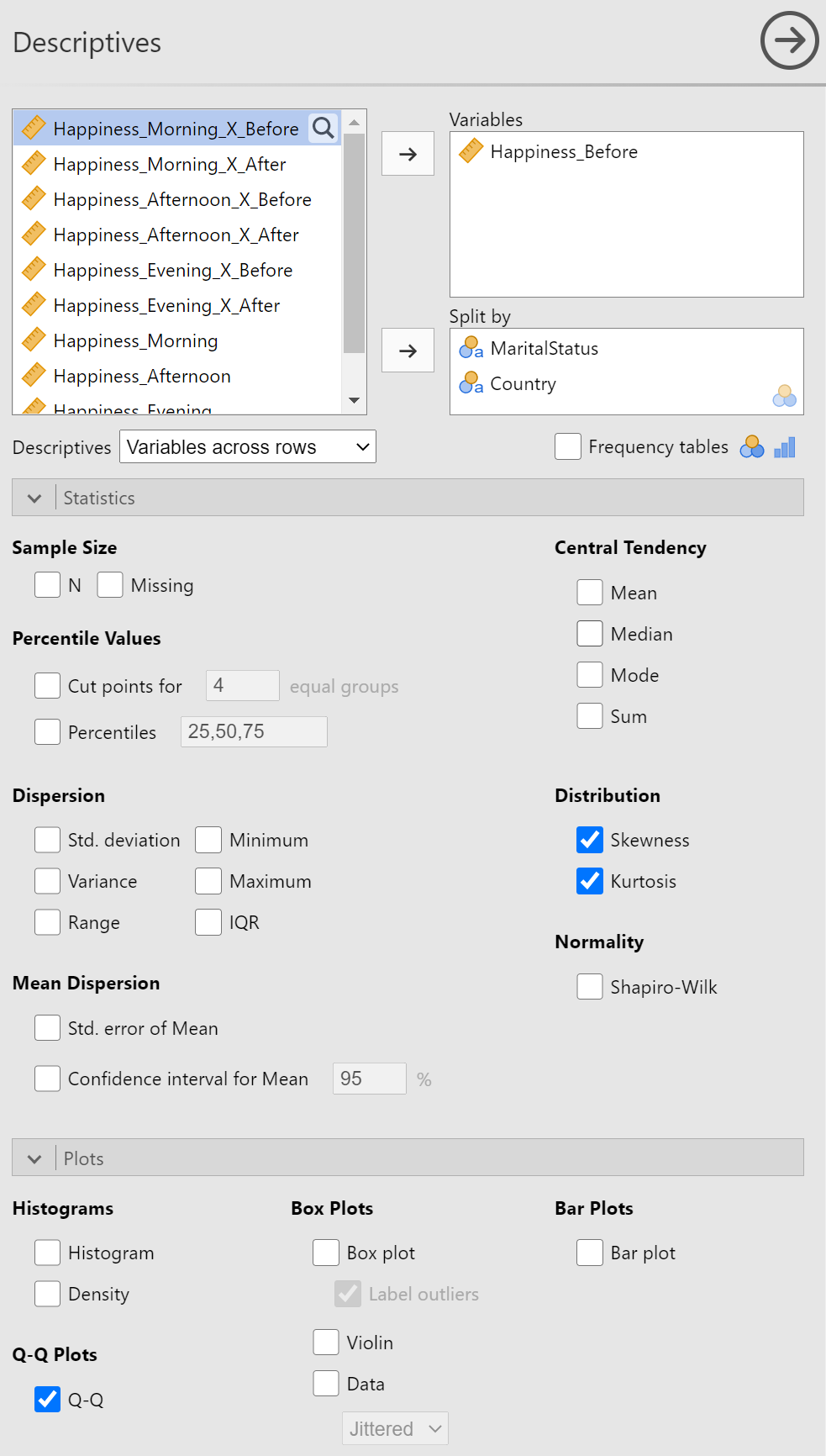
We’ll check for normality of the DV within each group by splitting the data by the between-subjects when we calculate skewness, kurtosis, and make our Q-Q plots. Figure 4 shows the complete setup for the descriptive statistics. To see each step individually, please review earlier posts.
Figure 4
Descriptives Panel Setup to Check Assumption of Normality
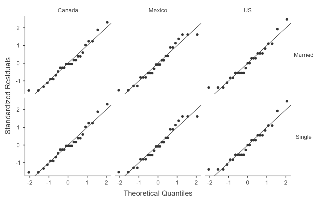
A quick review of the skewness and kurtosis values in table 11 reveals that all are within 2 SE of the normal value of 0 and thus there is no violation of the assumption. The Q-Q plots in figure 5 similarly show that the data nicely align with the expected normal distribution.
Table 11
Skewness and Kurtosis Values Across Marital Status and Country of Origin
| Marital Status | Country | Skewness | SE | Kurtosis | SE |
|---|---|---|---|---|---|
| Married | Canada | 0.512 | 0.464 | 0.0455 | 0.902 |
| Mexico | 0.215 | 0.464 | -1.0014 | 0.902 | |
| US | 0.683 | 0.464 | 0.2837 | 0.902 | |
| Single | Canada | 0.512 | 0.464 | 0.0455 | 0.902 |
| Mexico | 0.215 | 0.464 | -1.0014 | 0.902 | |
| US | 0.683 | 0.464 | 0.2837 | 0.902 |
Figure 5
Q-Q Plots of Happiness Ratings (before training) by Marital Status and Country
Homogeneity of Variance
As you may recall from the one-way between-subjects ANOVA post, this assumption can be checked as part of the ANOVA procedure. Let's put a pin in this and revisit once the ANOVA output is generated.
Setting up the Factorial Between-Subjects ANOVA
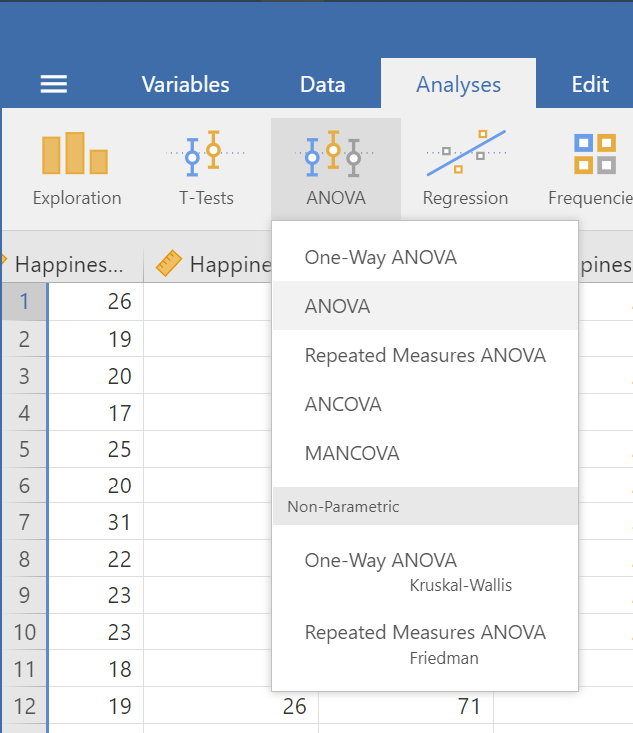
To start the ANOVA procedure, click on the "ANOVA" button in the "Analyses" tab then select "ANOVA" from the menu (see figure 6).
Figure 6
Selecting ANOVA procedure from Analyses Tab
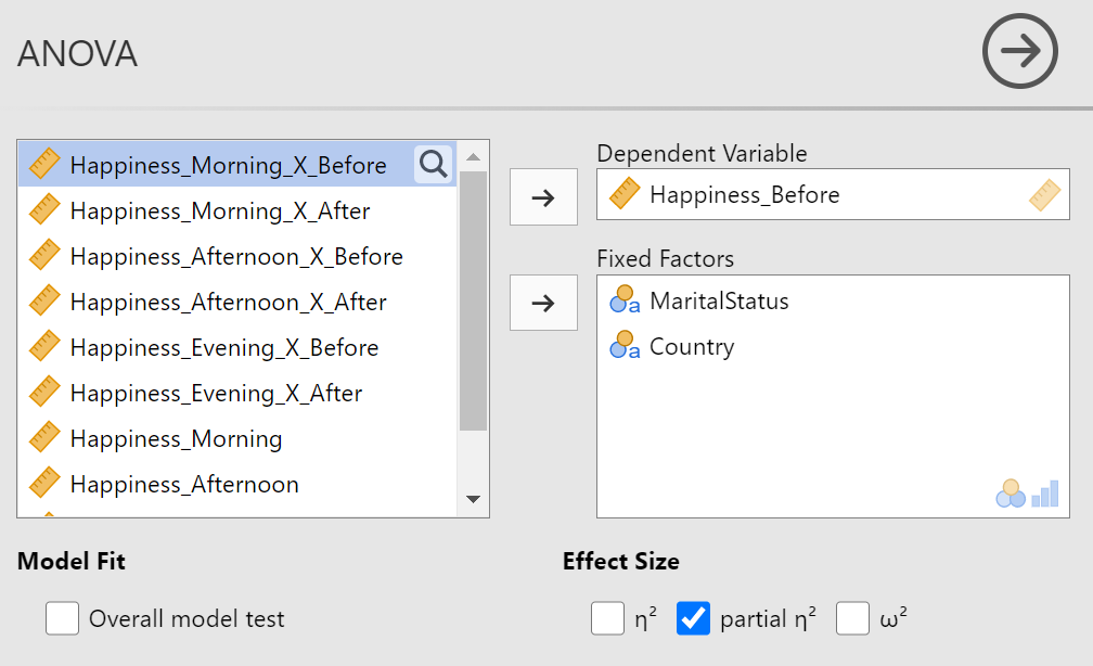
In the first panel of the ANOVA options, drag your outcome variable (i.e., "Happiness_Before" in our example) to the "Dependent Variable" box. Next, drag the two, between-subjects, predictors to the "Fixed Factors" box. Lastly, check the "partial η2" option. Figure 7 shows the completed panel.
Figure 7
Completed Top Panel for Factorial Between-Subjects ANOVA
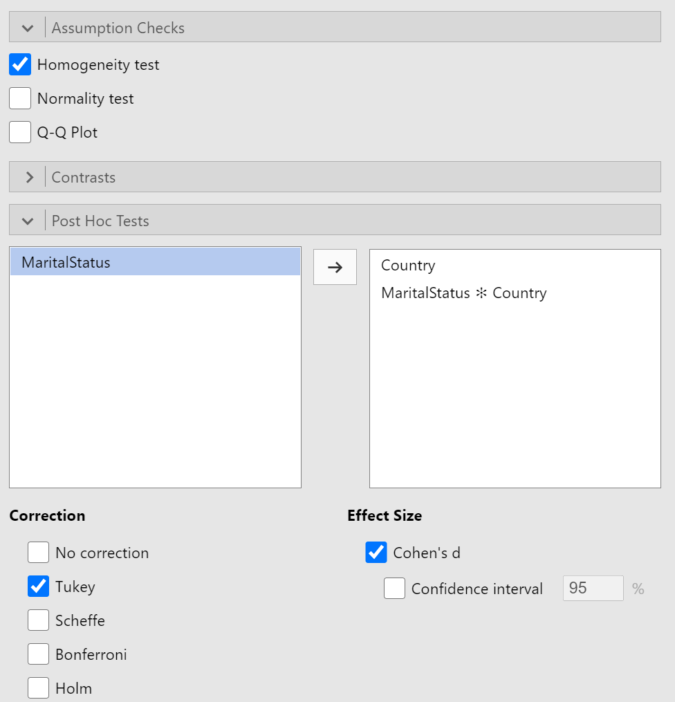
Next you'll want to turn on the "Homogeneity test" option under "Assumption Checks". When you get to the "Post Hoc Tests" section, pause and think about which make sense for follow-up tests. That is, which have more than two levels? Effects that only include two levels do not require a post hoc test because the ANOVA already indicates that the pairwise comparison is statistically significant. For those effects (like "Marital Status" in this example), you can simply look at the marginal means to interpret the significant effect. Also, by definition, any interaction term will have more than two levels because each variable in the interaction term must have at least 2 levels. Figure 8 shows the completed "Assumption Checks" section and the "Post Hoc Tests" section.
Figure 8
Completed Assumption Checks and Post Hoc Tests Sections
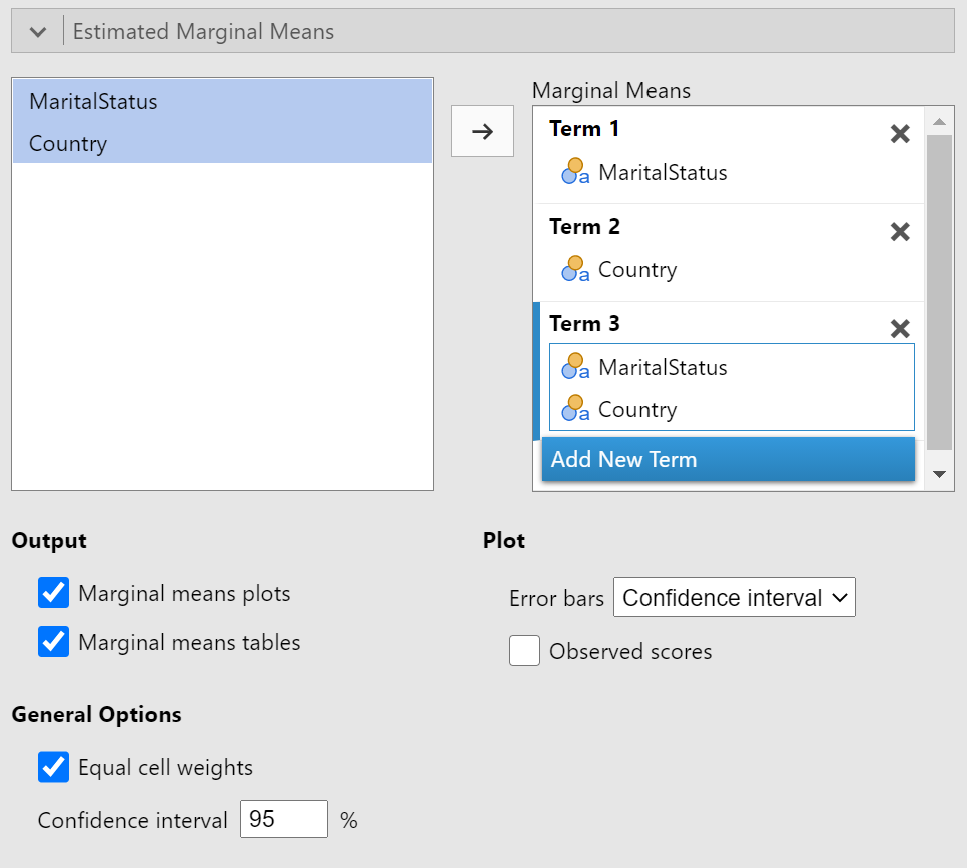
Last step for our set up is to request the estimated marginal means in tables and figures. This is a little more involved than we've done previously because we have to tell jamovi which variables we want included and how we want them organized. Essentially, we want to replicate the set up from our design. We want a term for each main effect and a term for each interaction effect. To get main effect estimated marginal means, simply drag a variable from the box on the left to the box on the right (e.g., under term 1). Click on the "Add New Term" button then drag the other predictor variable to the box under "Term 2" (see figure 9).
Figure 9
Creating a New Term for Estimated Marginal Means
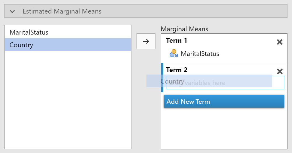
To calculate the estimated marginal means for the interaction term, click "Add New Term" then drag both predictors to the "drag a variable here" box under the "Term 3" header. For the output, I suggest that you turn on "Marginal means tables" in addition to what is already selected (i.e., "Marginal means plots","Equal cell weights"). Figure 10 shows the completed "Estimate Marginal Means" panel.
Figure 10
Completed Estimated Marginal Means Panel
We're now ready to review the output!
Reviewing the output for the Factorial Between-Subjects ANOVA
Homogeneity of Variance Check
Although the ANOVA table is the first part of the output for this set of analyses, we really need to check on the assumption of equality of error variances using Levene's test. The results of this test are reproduced in table 12.
Table 12
Levene's Test for Homogeneity of Variance
| F | df1 | df2 | p |
|---|---|---|---|
| 0.375 | 5 | 144 | 0.865 |
The p-value for this test is 0.865 which is above our threshold for rejection (α = 0.05) so we should maintain our assumption of the homogeneity of error variance.
Now for the main show: the ANOVA table!
ANOVA Table
The tests for our main effects and interaction effect are all within the table at the top of the "ANOVA" section (see table 13).
Table 13
Between-Subjects ANOVA Table
| Effect | Sum of Squares | df | Mean Square | F | p | η2p | |
|---|---|---|---|---|---|---|---|
| Marital Status | 0 | 1 | 0.0 | 0 | 1.000 | 0.000 | |
| Country | 47939 | 2 | 23969.3 | 1381 | < .001 | 0.950 | |
| Marital Status ✻ Country | 0 | 2 | 0.0 | 0 | 1.000 | 0.000 | |
| Residuals | 2499 | 144 | 17.4 |
A quick scan of the table reveals some interesting results. Primarily, the sum of squares for Marital Status and for the interaction of Marital Status and Country are 0. This means that there was no difference in these cell means! This is a clear clue that our data have been created rather than recorded! That being the case, we can still follow through with our procedure, just as if our data were not falsified.
The only effect in which we have some confidence in rejecting the null hypothesis is for "Country" because it has a p-value of < .001 and a very large effect size of η2p = 0.950. Because "Country" includes three levels (i.e., "Canada", "US", and "Mexico"). We will need to check the post hoc test to determine which countries had different levels of happiness before mindfulness training.
Post Hoc Tests
The pairwise comparisons using Tukey HSD are presented in table 14.
Table 14
Tukey HSD Comparisons for Levels of Country
| Country | Country | Mean Difference | SE | df | t | ptukey | Cohen's d | |
|---|---|---|---|---|---|---|---|---|
| Canada | - | Mexico | -16.1 | 0.833 | 144 | -19.3 | < .001 | -3.87 |
| - | US | 27.2 | 0.833 | 144 | 32.6 | < .001 | 6.53 | |
| Mexico | - | US | 43.3 | 0.833 | 144 | 52.0 | < .001 | 10.40 |
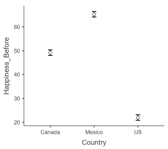
This table indicates that each country was statistically significantly different (ps < .001) and all have huge effect sizes (ds > |3.86|). These results are reinforced in the estimated marginal means plot because the 95% CI error bars do not (see figure 11).
Figure 11
Error Bar Plot of Happiness (Before Training) by Country

We can get the exact values for the means and confidence interval bounds from the estimated marginal means table (see table 15).
Table 15
Estimated Marginal Means of Happiness by Country
| Country | Mean | SE | 95% CI Lower | 95% CI Upper |
|---|---|---|---|---|
| Canada | 49.2 | 0.589 | 48.0 | 50.4 |
| Mexico | 65.3 | 0.589 | 64.2 | 66.5 |
| US | 22.0 | 0.589 | 20.8 | 23.2 |
As we saw in figure 11, Mexico had the highest rating followed by Canada and US last.
Before we leave the results section. I want us to peak at that non-significant interaction. Figure 12 is the interaction plot of Marital Status X Country.
Figure 12
Interaction Plot of Marital Status x Country
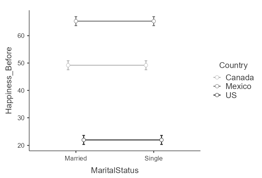
Notice how the lines between "Married" and "Single" are flat. This shows that there is now change in happiness across marital status within each level of country. Non-parallel lines in an interaction plot suggest an interaction. The formal test (as part of the ANOVA) will tell us if the deviation from no interaction (i.e., slope is 0) is sufficient to warrant a rejection of the null hypothesis.
The Write-Up of The Factorial Between-Subjects ANOVA
A reminder of the the pieces of our write-up.
- Assumptions
- ANOVA
- Post hoc tests
Within each of these, we need to:
- State the test/analysis
- Explain what we've found
- Provide statistical evidence.
Here's the example:
"To check the assumption of normality for the factorial between-subjects ANOVA, I split my outcome variable of Happiness (before training) by Country and Marital Status then calculated skewness and kurtosis values. The results suggest that there is no violation of the assumption because all skewness and all kurtosis values are within 2 SE of 0 (see table 1). I checked the assumption of homogeneity of variance using Levene's test. The test results suggest no violation of homogeneity of variance (F[5,144] = 0.375, p = 0.865). The factorial between-subjects ANOVA was conducted using the ANOVA procedure in jamovi. The ANOVA results are presented in table 2. There interaction of marital status by country and the main effect of marital status were not statistically significant (ps = 1.00) but the main effect of county was very large and statistically significant (F[2,144] = 1381, p < . 001, η2p = 0.950). Tukey HSD post hoc comparisons revealed that all countries had significantly different happiness ratings before training (see table 3). An error bar plot of estimated marginal means suggest that Mexico (M = 65.3, 95% CI [64.2,66.5]) had the highest happiness rating followed by Canada (M = 49.2, 95% CI[48.0, 50.4]), and then the US (M = 22, 95% CI[20.8,23.2]).See figure 1."
Table 1
Skewness and Kurtosis Values Across Marital Status and Country of Origin
| Marital Status | Country | Skewness | SE | Kurtosis | SE |
|---|---|---|---|---|---|
| Married | Canada | 0.512 | 0.464 | 0.0455 | 0.902 |
| Mexico | 0.215 | 0.464 | -1.0014 | 0.902 | |
| US | 0.683 | 0.464 | 0.2837 | 0.902 | |
| Single | Canada | 0.512 | 0.464 | 0.0455 | 0.902 |
| Mexico | 0.215 | 0.464 | -1.0014 | 0.902 | |
| US | 0.683 | 0.464 | 0.2837 | 0.902 |
Table 2
Between-Subjects ANOVA Table
| Effect | Sum of Squares | df | Mean Square | F | p | η2p | |
|---|---|---|---|---|---|---|---|
| Marital Status | 0 | 1 | 0.0 | 0 | 1.000 | 0.000 | |
| Country | 47939 | 2 | 23969.3 | 1381 | < .001 | 0.950 | |
| Marital Status ✻ Country | 0 | 2 | 0.0 | 0 | 1.000 | 0.000 | |
| Residuals | 2499 | 144 | 17.4 |
Table 3
Estimated Marginal Means of Happiness by Country
| Country | Mean | SE | 95% CI Lower | 95% CI Upper |
|---|---|---|---|---|
| Canada | 49.2 | 0.589 | 48.0 | 50.4 |
| Mexico | 65.3 | 0.589 | 64.2 | 66.5 |
| US | 22.0 | 0.589 | 20.8 | 23.2 |
Figure 2
Error Bar Plot of Happiness (Before Training) by Country
