Factorial Within-Subjects Analysis of Variance (ANOVA)
Factorial Within-Subjects Analysis of Variance (ANOVA)Revisiting the Within-Subjects DesignAssumptionsA Factorial Within-Subjects ExampleOrder of AnalysesThe Factorial Within-Subjects ANOVAInterpreting EffectsReporting Post Hoc AnalysesUsing jamovi Repeated Measures ANOVA for the Factorial Within-Subjects ANOVAThe Data SetThe Research QuestionChecking AssumptionsNormalitySphericitySetting up the Repeated Measures ANOVASetting up the VariablesAssumption ChecksPost Hoc TestsEstimated Marginal MeansInterpreting the ResultsThe ANOVA TablePost Hoc TestEstimated Marginal MeansThe Write-Up
Revisiting the Within-Subjects Design
The within-subjects, or repeated measures, design involves administering the various level of independent variables to the same sample of individuals. Because we are able to account for regularities stemming from the participants, we can account for and remove that source of variation from our error term. This reduction in error results in increased statistical power.
Assumptions
We will need to check two assumptions, just as we had for the one-way within-subjects ANOVA.
- Normality of DV within each combination of levels of IVs
- Sphericity or equality of variance across difference scores.
A Factorial Within-Subjects Example
Let’s start off with a 3x2 within-subjects design example. By refering to our design as “3x2” indicates that we have two independent variables. The first has 3 levels and the second has 2 levels. The within-subjects name indicates that each participant will receive all levels of all IVs (and have a dependent variable score associated with each administration).
Here’s the set up. A sensation and perception psychologist is investigating the impact of lighting color (natural, green, and red) and intensity (bright and dim) on flavorfulness ratings of vegetables (100 point scale). The researcher invites 5 children to participate in six conditions. The split-plot table is presented in Table 1.
Table 1
Split Plot Design of Example
| Color | |||
|---|---|---|---|
| Intensity | Natural | Green | Red |
| Dim | P1 = 69 | P1 = 84 | P1 = 31 |
| P2 = 69 | P2 = 84 | P2 = 39 | |
| P3 = 69 | P3 = 84 | P3 = 39 | |
| P4 = 73 | P4 = 88 | P4 = 35 | |
| P5 = 74 | P5 = 89 | P5 = 45 | |
| Bright | P1 = 79 | P1 = 68 | P1 = 52 |
| P2 = 79 | P2 = 70 | P2 = 62 | |
| P3 = 81 | P3 = 71 | P3 = 63 | |
| P4 = 80 | P4 = 72 | P4 = 56 | |
| P5 = 84 | P5 = 71 | P5 = 64 | |
Our 3x2 design could be conceptualized as a 3x2x5 design because we are analyzing the variability in flavor scores due to our participants. We will be removing this source of variance rather than examining it for statistical significance. Therefore we do not participant in our description.
Order of Analyses
With our dat set laid out, we can think about the types and number of effects we will want to test in our within-subjects ANOVA. We will want to test for each main effect and for the interaction effect.
Determining Number of Effects
Include all Main Effects.
- There will be one main effect for each independent variable.
- In the Vegetable Flavor example, we have two IV: color and light.
Find Unique Combinations of IV for Interaction Effects.
- Eliminate and interaction effects that contain the same factors as another interaciton.
- Color x Light is the same as Light x Color, so there is only one interaction effect.
The Factorial Within-Subjects ANOVA
When we’re done with checking our assumptions, we run the ANOVA. The ANOVA always precedes the post hoc analyses because it controls for the increased Type I error that accompanies multiple testing.
We’ll run through the SPSS procedure to produce the factorial within-subjects ANOVA using the repeated measures general linear model in the next section, for now we’ll review the interpretation steps. Table 2 is the ANOVA table that results from the repeated measures GLM for our example.
Table 2
Within-Subjects ANOVA Table
| Source | Sum of Squares | df | Mean Square | F | p |
|---|---|---|---|---|---|
| Color | 5368.067 | 1.06 | 5044.375 | 199.556 | .000 |
| Error(color) | 107.600 | 4.257 | 25.278 | – | – |
| Intensity | 213.333 | 1 | 213.333 | 51.200 | .002 |
| Error(Intensity) | 16.667 | 4 | 4.167 | – | – |
| Color*Intensity | 1786.067 | 1 | 893.033 | 1448.162 | .000 |
| Error(Color*Intensity) | 4.933 | 4 | .617 | – | – |
Note. Degrees of freedom for Color and color*intensity adjusted for sphericity violation using Greenhouse-Geisser correction.
You should notice a few things. First, as indicated by the table note, there was a violation of the assumption of sphericty an that the degrees of freedom were adjusted using the Greenhouse-Geisser correction. Second, there are error terms associated with each effect. That is, we are required to calculated a separate demoninator for each main effect and for the interaction effect.
The need for separate error terms stems from how are grouping our sources of variance. Recall that the error term in our F-statistics represents variability in individual scores about the group means for which we cannot account. In a within-subjects design, we are calculating how the participants’ scores vary from their means and remove that variability from our error term. The reason why this leads to different error terms is because we will have different sets of scores involved in each effect.
Interpreting Effects
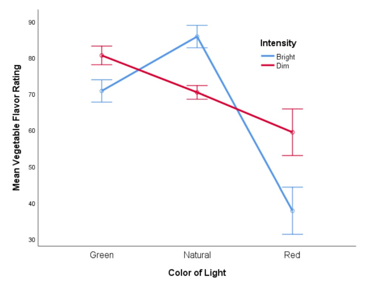
Table 1 reveals a significant interaction effect so we will focus our interpreation around that effect. Let’s look to the interaciton plot to guide our interpretation. Figure 1 is a line chart of the effect of color and intensity on reported vegetable flavor.
Figure 1
Interaction Line Graph of Color and Intensity on Vegetable Flavor
Note. Error bars represent 95% CI.
This looks like a busy chart but let’s look for patterns and violations of patterns to guide our interpretation. The first pattern I notice is the nice straight line for the dim lighting conditon. That is, the flavor rating is highest for the green colored light, lowest for the red colored light, and in the middle for natural lighting. I’ll use that straight line as my reference as I examine what is happening in the bright lighting condition.
Recall that a significant interaction tells us that something in the relationship between one IV and the DV changes when we apply the levels of the other IV. As such, we should be looking for where our relationship (i.e., the straight line in the dim condition) changes.
The bright lighting condition does not show the same straight line but rather the highest flavor rating is for natural light rather than green light. Importantly, however, notice that the flavor rating for the green colored light is lower than that of the green colored light in the dim condition just as the red colored light leads to a lower rating than that of the red colored light in the dim condition. Stated another way, we would expect the natural colored light in the bright condition to behave in a similar way to that of the natural colored light in the dim condition (i.e., produce an average flavor rating), but it does not. This deviation from expectation is what is driving our interaction effect and thus we should focus or write-up on that feature.
Reporting Post Hoc Analyses
To corroborate our interpration of the interaction plot, we’ll want some statistics. Just as we had in the one-way within-subjects ANOVA, we will utilize the Bonferroni correction. We do have the option of performing simple effects tests as well. If we were to perform them, I would suggest that we narrow in on the interesting changing happening in the natural light conditions. However, given that we perform the Bonferroni correction for multiple post hoc paired samples t-tests, it makes sense to jump to those corrections now. Table 3 provides the means and confidence intervals for flavor rating at the interaction of the IVs.
Table 3
Means and Bonferroni-adjusted Confidence Intervals
| Color | Intensity | Mean | 95% CI LL | 95% CI UL | |
|---|---|---|---|---|---|
| Green | Bright | 70.800 | 67.708 | 73.892 | |
| Dim | 80.600 | 78.025 | 83.175 | ||
| Natural | Bright | 85.800 | 82.708 | 88.892 | |
| Dim | 70.400 | 68.517 | 72.283 | ||
| Red | Bright | 37.800 | 31.324 | 44.276 | |
| Dim | 59.400 | 52.972 | 65.828 |
Note. Confidence intervals adjusted using Bonferroni correction.
With these means and confidence intervals, we can provide a succinct description of the interaction.
“The interaction plot in Figure 1 suggests that a trend of flavor ratings decreasing from green light, to natural light, to red light in the dim condition was different for the bright condition. Although the flavor ratings in green and red lights are reliable lower in the bright than dim condition (see Bonferroni-corrected 95% CI in Table 3), the trend reverses for the natural light condition. That is ratings are reliably higher higher in the bright condition than the dim condition for natural light (see Table 3).”
Using jamovi Repeated Measures ANOVA for the Factorial Within-Subjects ANOVA
We're back to the Repeated Measures ANOVA procedure for this factorial within-subject ANOVA and we'll stay here for the mixed factorial ANOVA, too.
The Data Set
I will continue to use my teaching example data set that I have used for the previous walk throughs. This will be very similar to the data set provided to you.
The Research Question
For this post, we'll try to answer "how does the time of day and the timing of mindfulness training impact happiness ratings?" As such, we'll be including our within-subjects variables to assess our outcome variable.
Checking Assumptions
We'll need to check our two assumptions for this within-subjects ANOVA: normality of the DV within each sample and sphericity, or the equality of error variance of difference scores.
Normality
We'll follow the typical pattern of checking our assumption of normality by calculating skewness and kurtosis values, and examining Q-Q plots.
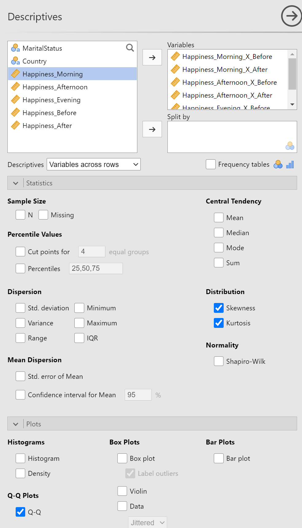
If you recall from the one-way within-subjects ANVOA, we'll need to include each of our samples, which have been separated into combinations of the within-subjects variables. For this example, we'll want to examine all variables that contain the outcome values with the combinations of the within-subjects variables (Hint: these are the variables in the data set that have "_X_") in the title. For each of these, we'll want "Skewness", "Kurtosis", and "Q-Q" options enabled. Figure 2 shows the completed descriptives panel.
Figure 2
Completed Descriptives Panel
A review of the skewness and kurtosis values (see table 4) indicates that all the skewness values are within 2 SE of 0 but that the kurtosis are up to 3.57 SE from 0. The Q-Q Plots (see figure 3) reveal the nature of the kurtosis is not severe enough to prevent the use of ANOVA.
Table 4
Skewness and Kurtosis Values of Happiness by Time of Day and Timing of Mindfulness Training
| Time of Day | Timing of Training | Skewness | SE | Kurtosis | SE |
|---|---|---|---|---|---|
| Morning | Before | -0.260 | 0.198 | -1.41 | 0.394 |
| After | -0.384 | 0.198 | -1.34 | 0.394 | |
| Afternoon | Before | -0.293 | 0.198 | -1.38 | 0.394 |
| After | -0.386 | 0.198 | -1.35 | 0.394 | |
| Evening | Before | -0.382 | 0.198 | -1.33 | 0.394 |
| After | -0.111 | 0.198 | -1.29 | 0.394 |
Figure 3
Q-Q Plots of Happiness by Time of Day and Timing of Mindfulness Training
| Before | After | |
|---|---|---|
| Morning | 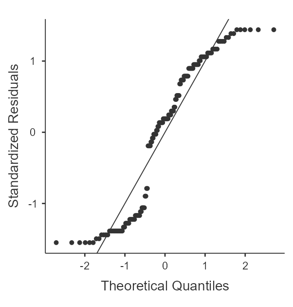 | 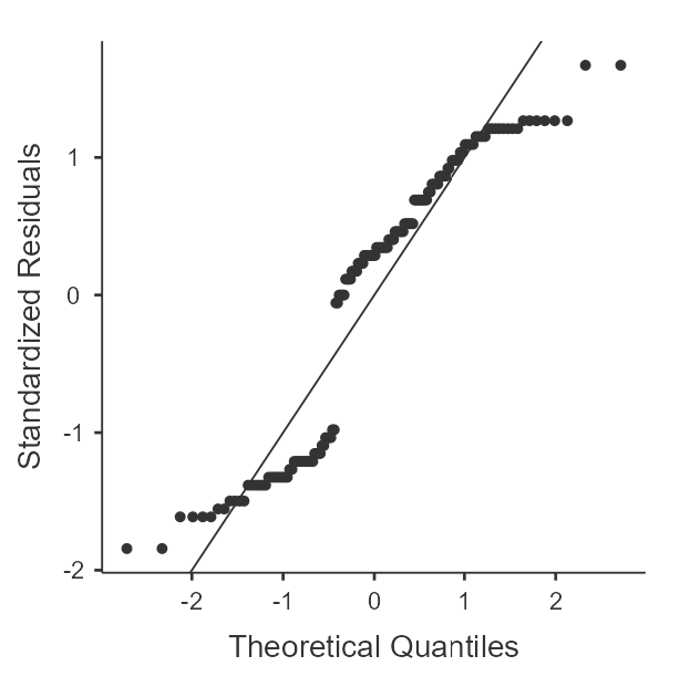 |
| Afternoon | 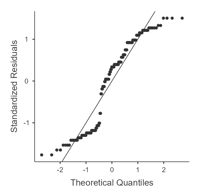 | 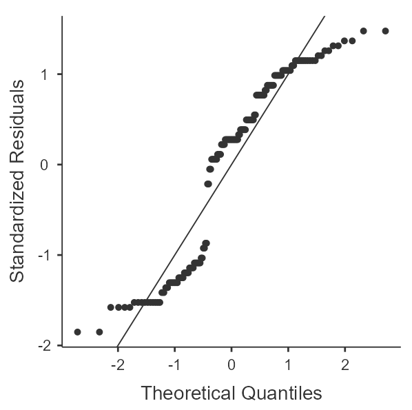 |
| Evening | 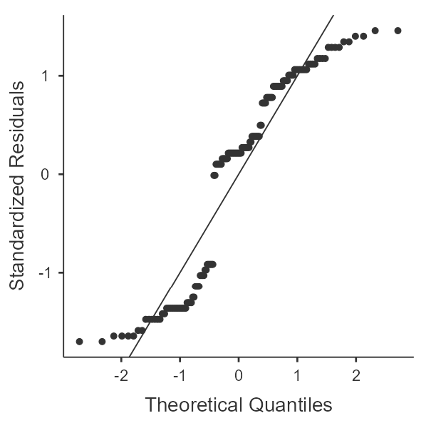 | 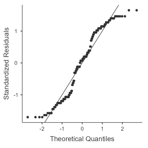 |
Sphericity
As before, we'll have to wait until we set up the repeated measures ANOVA to test the assumption of sphericity using Mauchly's test.
Setting up the Repeated Measures ANOVA
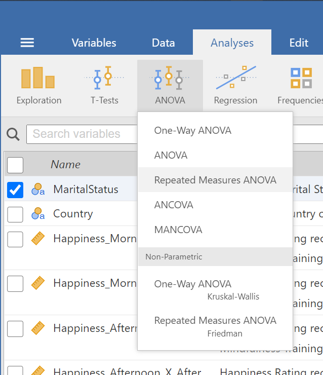
We'll need to get back to the Repeated Measures ANOVA under the ANOVA menu in the "Analyses" tab (see figure 4).
Figure 4
Repeated Measures Option under the ANOVA Menu in the Analyses Tab
Setting up the Variables
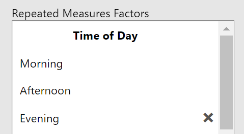
As we did with the one-way within-subjects ANOVA, we need to tell jamovi about our within-subjects variables and dependent variable because of the wide format of the data set. First, start by giving the name of the first within-subjects variable then add in each level (see figure 5).
Figure 5
First Within-Subjects Variable Setup
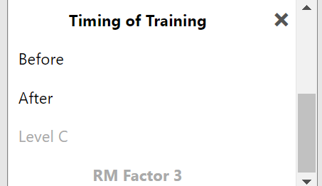
Repeat this process for the second within-subjects variable (see figure 6).
Figure 6
Second Within-Subjects Variable Setup
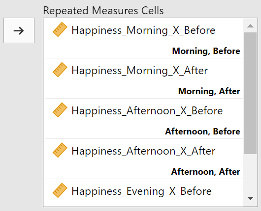
Now that jamovi knows about our within-subjects variables, we can align our data to these factors. Luckily for us, our variables are also labeled with these same factors (and in the correct order). Drag a variable from the box on the right to the corresponding combination of factors on the right. Figure 7 shows an example of the alignment.
Figure 7
Aligning Variables with Factors
The last steps for this area is to turn on our effect size (Partial η2) and label our dependent variable as "Happiness" (see figure 8).
Figure 8
Effect Size and DV Label

Let's move on to the "Assumption Checks" section.
Assumption Checks
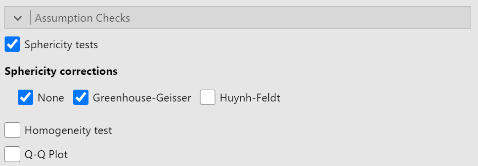
This section is fairly simple. We just need to turn on "Sphericity tests" and to also turn on "Greenhouse-Geisser" under "Sphericity corrections." (See figure 9)
Figure 9
Assumption Check Options
Post Hoc Tests
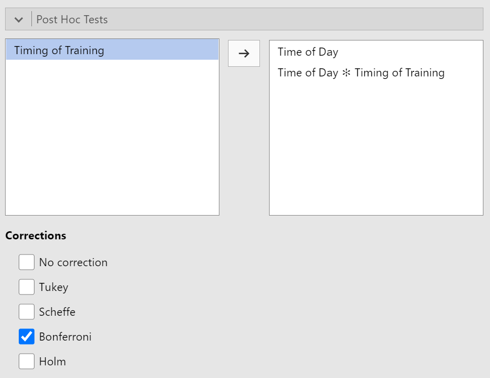
The post hoc tests sections requires two steps. First, we need to tell jamovi which comparisons we want to test. We need all the effects that involve more than two levels. This is "Time of Day" and the interaction of "Time of Day x Timing of Training." We don't need "Timing of Training" because it only has levels ("before" and "after").
Second, we need to switch the correction from "Tukey" to "Bonferroni." See Figure 10 for the complete setup for post hoc tests.
Figure 10
Post Hoc Tests Setup
We're almost there. Last output we need to generate are those related the estimated marginal means.
Estimated Marginal Means
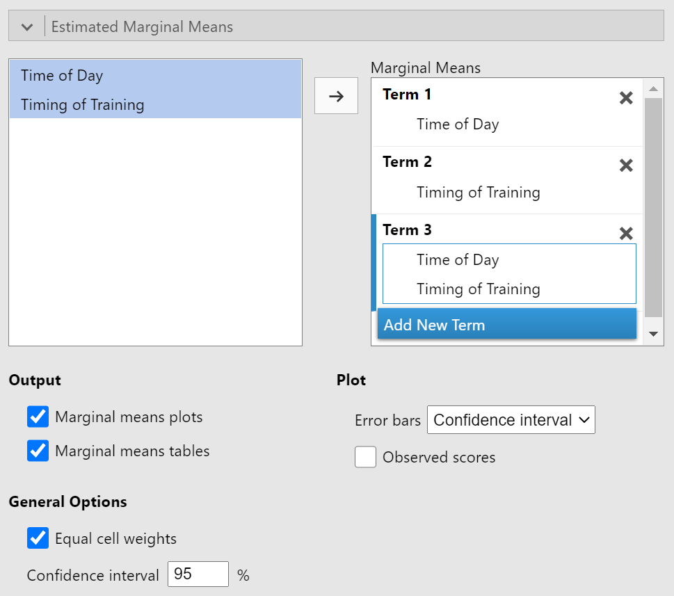
We'll want to get the marginal means for each within-subjects factor as well as the means for the interaction of those factors. Request these as both plots and means. You can see this set up in figure 11.
Figure 11
Estimated Marginal Means Setup
That's it! We've got everything set up for what we need so now we can review the output.
Interpreting the Results
Let's finish our assumption check of sphericity by reviewing Mauchly's test in Table 5.
Table 5
Mauchly's Test of Sphericity
| Effect | Mauchly's W | p | Greenhouse-Geisser ε | Huynh-Feldt ε | |
|---|---|---|---|---|---|
| Time of Day | 0.0629 | < .001 | 0.516 | 0.517 | |
| Timing of Training | 1.0000 | NaNa | 1.000 | 1.000 | |
| Time of Day ✻ Timing of Training | 0.3530 | < .001 | 0.607 | 0.610 |
a The repeated measures has only two levels. The assumption of sphericity is always met when the repeated measures has only two levels.
Unfortunately, we have a violation for both the main effect of "Time of Day" and for the interaction effect of "Time of Day x Timing of Training" (ps<.001). We'll need to use the "Greenhouse-Geisser" correction in the ANOVA table. You'll notice a "specific note" denoted as a in the table. It explains why we have "NaN" or "Not a Number" for the p-value for timing of training. Sphericity does not apply when there are only two levels involved. This is because sphericity is about equality of variance of difference scores and we can only have one set of differences scores and no others with which to compare.
The ANOVA Table
The ANOVA table is a lot bigger than it was in the one-way within-subjects ANOVA because there is a "residuals" term associated with each effect (see Table 6). I've removed the rows from the table where "Sphericity Correction" is "None" to make the table more concise.
Table 6
Repeated Measures ANOVA Table
| Within Subjects Effects | Sum of Squares | df | Mean Square | F | p | η²p | |
|---|---|---|---|---|---|---|---|
| Time of Day | 22984.1 | 1.03 | 22261.1 | 18.327 | < .001 | 0.110 | |
| Residual | 186857.9 | 153.84 | 1214.6 | ||||
| Timing of Training | 1959.5 | 1.00 | 1959.5 | 27.315 | < .001 | 0.155 | |
| Residual | 10689.1 | 149.00 | 71.7 | ||||
| Time of Day ✻ Timing of Training | 61.1 | 1.21 | 50.3 | 0.377 | 0.581 | 0.003 | |
| Residual | 24166.3 | 180.94 | 133.6 |
Note. Degrees of freedom adjusted using Greenhouse-Geisser correction
What's important in this table? As before, we want to check our confidence (i.e., the p-value) and effect size for each effect. The interaction effect was not statistically significant (p = 0.581) with a very small effect size. The main effects of "time of day" and "timing of training" were reliable (ps < .001) with small (d = .110 an d = .155, respectfully).
The next step is to conduct post-hoc analyses, but we only need to do that for "time of day". We already know that the two levels of "timing of training" are reliably different but we'll need to consult the marginal means to interpret this difference.
Post Hoc Test
The post-hoc comparisons using the bonferroni correction for "time of day" are presented in table 7.
Table 7
Post Hoc Comparisons
| Time of Day | Time of Day | Mean Difference | SE | df | t | pbonferroni | |
|---|---|---|---|---|---|---|---|
| Morning | Afternoon | -4.84 | 0.366 | 149 | -13.23 | < .001 | |
| Evening | -12.29 | 2.498 | 149 | -4.92 | < .001 | ||
| Afternoon | Evening | -7.45 | 2.483 | 149 | -3.00 | 0.010 |
As the table reveals, all levels are significantly different (ps < .01). Let's check out the marginal means to interpret the results in terms of the data presented.
Estimated Marginal Means
I like to look at the plots to help interpret the effects. Figure 12 is an error bar plot of happiness across levels of "time of day".
Figure 12
Error Bar Plot of Happiness Across Levels of Time of Day
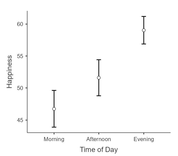
This plot indicates that individuals reported the greatest levels of happiness in the evening, followed by the afternoon, and then by the morning. Let's check out figure 13 for the error bar plot of happiness across timing of training.
Figure 13
Error Bar Plot of Happiness Across Timing of Training
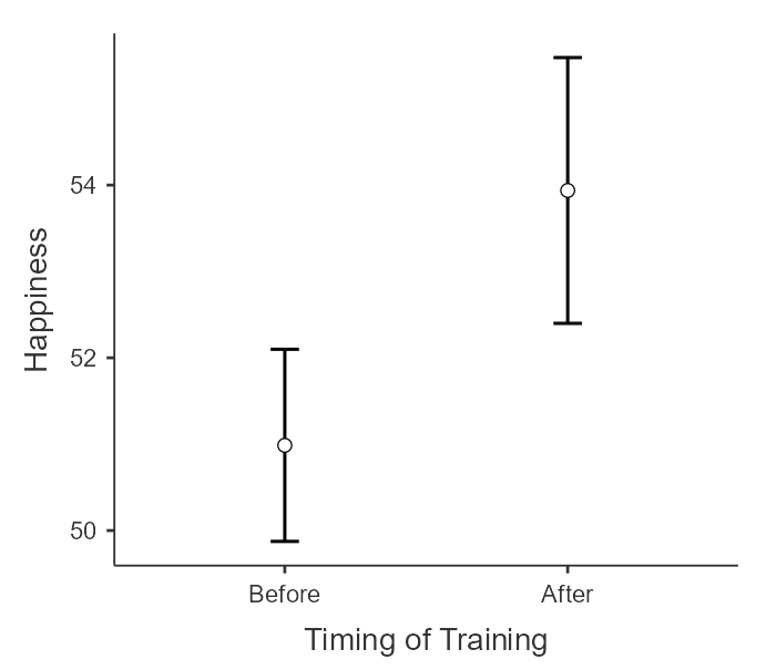
This plot informs us that individuals are reliably happier after mindfulness training than before.
The Write-Up
Let's put this all together in an APA-styled write-up.
"To answer the research question, I performed a factorial within-subjects ANOVA. I tested the assumption of normality of the outcome variable within each sample by calculating skewness and kurtosis values. A review of the skewness and kurtosis values (see table 4) indicates that all the skewness values are within 2 SE of 0 but that the kurtosis are up to 3.57 SE from 0. Although the kurtosis values are larger than 2 SE, this is not so extreme to influence the conclusion of the ANOVA so I will maintain the assumption of normality. The assumption of sphericity was checked using Mauchly's test. The test revealed violations for the interaction effect and the main effect (ps < .001) so I used the Greenhouse-Geisser correction for the Within-Subjects ANOVA. The ANOVA table with the Greehouse-Geisser corrections applied is presented in Table 2. This table reveals significant but small main effects but not a significant interaction effect. Bonferroni corrected pairwise comparisons for the effect of time of day revealed that all levels were reliably differ (see Table 3). An investigation of the estimated marginal means of time of day (figure 1) and timing of training (figure 2) reveal that individuals were happiest in the evening, followed by the afternoon, and then the morning. Individuals were also happier after training than before training."
Table 1
Skewness and Kurtosis Values of Happiness by Time of Day and Timing of Mindfulness Training
| Time of Day | Timing of Training | Skewness | SE | Kurtosis | SE |
|---|---|---|---|---|---|
| Morning | Before | -0.260 | 0.198 | -1.41 | 0.394 |
| After | -0.384 | 0.198 | -1.34 | 0.394 | |
| Afternoon | Before | -0.293 | 0.198 | -1.38 | 0.394 |
| After | -0.386 | 0.198 | -1.35 | 0.394 | |
| Evening | Before | -0.382 | 0.198 | -1.33 | 0.394 |
| After | -0.111 | 0.198 | -1.29 | 0.394 |
Table 2
Repeated Measures ANOVA Table
| Within Subjects Effects | Sum of Squares | df | Mean Square | F | p | η²p | |
|---|---|---|---|---|---|---|---|
| Time of Day | 22984.1 | 1.03 | 22261.1 | 18.327 | < .001 | 0.110 | |
| Residual | 186857.9 | 153.84 | 1214.6 | ||||
| Timing of Training | 1959.5 | 1.00 | 1959.5 | 27.315 | < .001 | 0.155 | |
| Residual | 10689.1 | 149.00 | 71.7 | ||||
| Time of Day ✻ Timing of Training | 61.1 | 1.21 | 50.3 | 0.377 | 0.581 | 0.003 | |
| Residual | 24166.3 | 180.94 | 133.6 |
Table 3
Post Hoc Comparisons
| Time of Day | Time of Day | Mean Difference | SE | df | t | pbonferroni | |
|---|---|---|---|---|---|---|---|
| Morning | Afternoon | -4.84 | 0.366 | 149 | -13.23 | < .001 | |
| Evening | -12.29 | 2.498 | 149 | -4.92 | < .001 | ||
| Afternoon | Evening | -7.45 | 2.483 | 149 | -3.00 | 0.010 |
Figure 1
Error Bar Plot of Happiness Across Levels of Time of Day

Figure 2
Error Bar Plot of Happiness Across Timing of Training

This plot informs us that individuals are reliably happier after mindfulness trainin