Mixed Factorial Analysis of Variance (ANOVA)
Mixed Factorial Analysis of Variance (ANOVA)Combining Between- and Within-Subjects FactorsAssumptionsA Mixed Factorial ExampleUsing jamovi Repeated Measures ANVOA for the Mixed Factorial ANOVAThe Data SetThe Research QuestionChecking AssumptionsNormalityHomogeneity of VarianceSphericitySetting up the Repeated Measures ANOVASetting up the VariablesAssumption ChecksPost Hoc TestsEstimated Marginal MeansInterpreting the ResultsChecking AssumptionsThe ANOVA TablesPost Hoc TestsEstimated Marginal MeansThe Write-Up
Combining Between- and Within-Subjects Factors
The great benefit of the general linear model is the ability to account for various designs into a single statistical model. For this course, the pinnacle of this generality is the “mixed factorial ANOVA.” As the term “factorial” implies, we will be including multiple independent variables. The term “mixed” tells us that we will be combining both within- and between-subjects factors.
The best thing about ending the course on this topic is that it is almost all review. We really are just combining the two types of factorial ANOVAs already discussed.
We can see this with the assumptions.
Assumptions
The mixed factorial ANOVA has three assumptions that we’ll need to verify.
- Normality of DV within each combination of levels of IVs. This was a common assumption for both between- and within-subjects designs.
- Homogeneity of variance for between-subjects IVs. This will appear slightly differently than before because we will have to check this assumption for across the DV scores in each level of the wtihin-subjects factor.
- Sphericity or equality of variance within-subjects IV. As in the original within-subjects ANOVA, we’ll want to verify that the difference scores across the combined levels of the variables are roughly equal.
A Mixed Factorial Example
Here is an example data set that involves the changes to SAT scores across the number of test attempts and the impact of a music education background. Table 1 shows a sample of a data set to illustrate the design.
Table 1
Split Plot Design of Example
| Test Attempt | |||
|---|---|---|---|
| Music Background? | First | Second | Third |
| Yes | P1 = 1261 | P1 = 1349 | P1 = 1415 |
| P2 = 1275 | P2 = 1361 | P2 = 1430 | |
| P3 = 1232 | P3 = 1316 | P3 = 1384 | |
| P4 = 1314 | P4 = 1396 | P4 = 1470 | |
| P5 = 1238 | P5 = 1326 | P5 = 1390 | |
| No | P6 = 1216 | P6 = 1221 | P6 = 1223 |
| P7 = 1179 | P7 = 1181 | P7 = 1182 | |
| P8 = 1188 | P8 = 1190 | P8 = 1192 | |
| P9 = 1181 | P9 = 1186 | P9 = 1185 | |
| P10 = 1203 | P10 = 1210 | P10 = 1211 | |
Note. Scores in table represent SAT scores
Pay particular attention to the participants. The same participants are in all three attempts for having no music education background but another group of participants are in the three attempts without having a music education background. As such, "Music" background is a between-subjects variable (with two levels) and "Test Attempt" is a within-subjects variable (with three levels). This is a 2 x 3 mixed factorial design.
The difference in participants will be important when we calculate (or rather, have jamovi calculate) the error terms.
Using jamovi Repeated Measures ANVOA for the Mixed Factorial ANOVA
The Data Set
For the final time for the course, I'll be using the example I have for the other sections. Please follow along using the dataset I provided you.
The Research Question
For this mixed factorial ANOVA example, we'll need one between-subjects variable and one within-subjects variable. I will investigate how country of origin (the between-subjects variable with three levels) and timing of mindfulness training (the within-subject variable with two levels) impacts happiness ratings.
Checking Assumptions
Normality
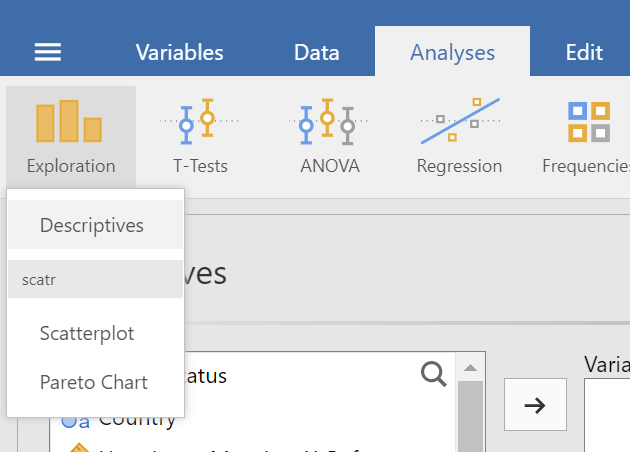
I'll continue to check for normally distributed outcomes scores within each sample with skewness and kurtosis values coupled with Q-Q plots. Start a new descriptive statistics section by clicking on the "Analyses" tab, then the "Exploration" menu and selecting "Descriptives" (see figure 1).
Figure 1
Descriptives from the Exploration Menu in the Analyses Tab
We will need to combine our approaches for between- and within-subjects designs. Drag the variables that contain the outcome scores for the levels of the within-subjects variable to the "Variables" box then drag the between-subjects variable to the "Split by" box. Turn on the "Skewness" and "Kurtosis" option under the "Distribution" area of the "Statistics" section. Lastly, turn on the "Q-Q" option in the "Q-Q Plots" area of the "Plots" section. Figure 2 shows the complete panel set up.
Figure 2
Completed Descriptives Panel Setup
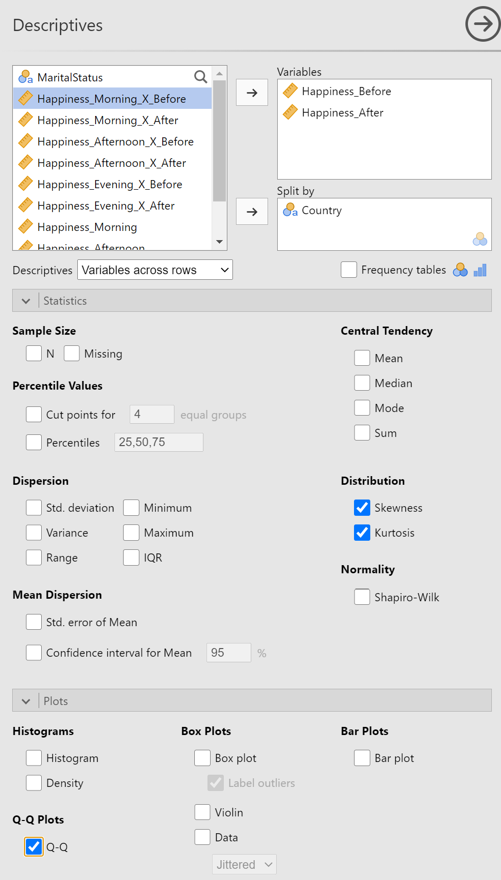
Table 1
Skewness and Kurtosis Values for Happiness Ratings by Timing of Training and Country
| Timing of Training | Country | Skewness | SE | Kurtosis | SE |
|---|---|---|---|---|---|
| Before | Canada | 0.496 | 0.337 | -0.0844 | 0.662 |
| Mexico | 0.208 | 0.337 | -1.0248 | 0.662 | |
| US | 0.661 | 0.337 | 0.1296 | 0.662 | |
| After | Canada | -0.487 | 0.337 | -0.5664 | 0.662 |
| Mexico | 0.440 | 0.337 | 0.0999 | 0.662 | |
| US | -0.630 | 0.337 | 0.2317 | 0.662 |
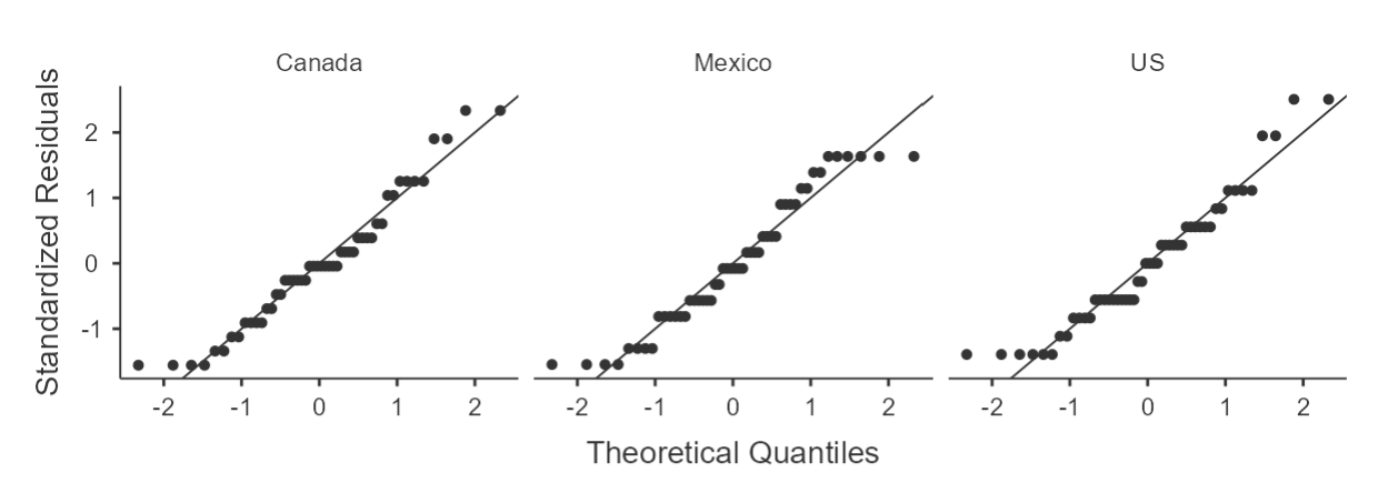
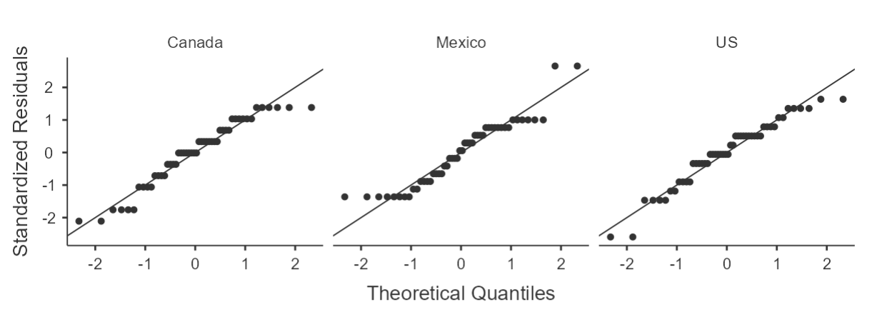
It seems that all values are within the 2 SE range for acceptable results under the assumption of normality. The Q-Q plots (see figure 3) reinforce this as most of the data are close to the reference line, except for Mexico after training, but that was not severe enough to overturn our assumption.
Figure 3
Q-Q Plots for Happiness Ratings by Timing of Training and Country
A) Before Training
B) After Training
Homogeneity of Variance
We'll need to wait to check this assumption as the test is an option in the Repeated Measures ANOVA setup.
Sphericity
This is an assumption we don't have to worry about this time because the within-subjects variable only has two levels. As such, sphericity does not apply.
Setting up the Repeated Measures ANOVA
Setting up the Variables
We are going to follow the same set up as we had for the factorial within-subjects ANOVA but add the between-subjects variable into the mix. Start by labeling the within-subjects factor in the "Repeated Measures Factors" box. Add a label for each level in the spaces below. You can now add the appropriate variables that contain the outcome variable within each level of the within-subjects variable to the "Repeated Measures Cells". Next, drag your between-subjects variable to the "Between-subjects Factors" box. Be sure to provide an appropriate label in the "Default Variable Label" box and to turn on "Partial η2" under the "Effect Size" options. The completed top portion of the Repeated Measures ANOVA panel is in figure 4.
Figure 4
Completed Top Portion of Repeated Measures ANOVA Panel

Assumption Checks
In the "Assumption Checks" section, you'll only need to enable the "Homogeneity test" option as sphericity does not apply.
Post Hoc Tests
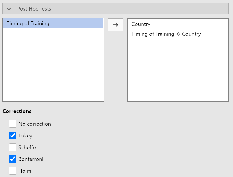
Next to Post Hoc Tests to determine which samples are reliably different from other samples. You'll want to drag over any effects that include more than two samples. In this example, that will be the between-subjects factor and the interaction term.
You may remember that for within-subjects variables, we use the "Bonferroi" correction but for the between-subjects variables, we use the "Tukey" correction. Simply enable both to get the correct output for each test. We will continue to read the "Tukey" p-value for the between-subjects tests but we'll use the "Bonferroni" p-value for the interaction effect (because it has within-subjects samples). Figure 5 depicts the completed post hoc tests section.
Figure 5
Completed Post Hoc Tests Section
Estimated Marginal Means
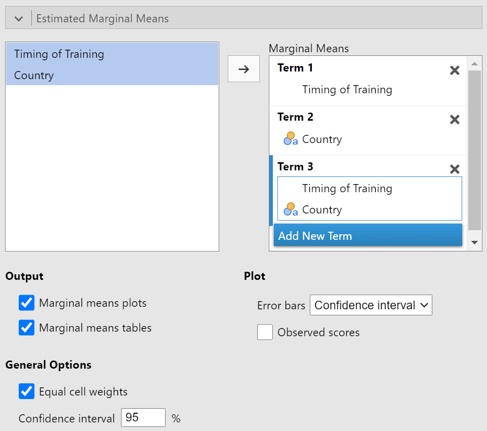
To get the details (i.e., means and 95% CI) for each sample, we'll need to set up our marginal means. Drag the within-subjects variable to the box under "Term 1." Click "Add New Term" then drag the between-subjects variable to the box under "Term 2." Click "Add New Term" one more time and drag both variables to the box under "Term 3". Turn on "Marginal means tables" in addition to "Marginal means plots," which should already be enabled. See figure 6 for the completed "Estimated Marginal Means" section
Figure 6
Completed Estimated Marginal Means Section
We have finished the setup of the mixed factorial ANOVA so let's check out the results
Interpreting the Results
Checking Assumptions
We left off with our assumption of homogeneity of variance. In mixed factorial design, we'll need to check that assumption within each level of the within-subjects variable. That is, we want to check if we have roughly equal variance across of between-subjects levels in each of our samples of within-subjects variable levels. Table 2 contains the two Levene's tests of homogeneity of variance.
Table 2
Levene's Tests of Homogeneity of Variance
| Timing of Training | F | df1 | df2 | p |
|---|---|---|---|---|
| Before | 0.957 | 2 | 147 | 0.386 |
| After | 4.625 | 2 | 147 | 0.011 |
It seems that we have a violation in happiness ratings after training but we can maintain the assumption for happiness before training. This is likely stemming from the issue with kurtosis in happiness ratings in Mexico after training (see figure 3, panel B). However, because we have large samples and equal sample sizes, our ANOVA is quite robust against this violation.
The ANOVA Tables
For a mixed factorial ANOVA in jamovi, we will have two ANOVA tables, one for the within-subjects effects (including any interaction terms that involve a within-subjects factor) and one for the between-subjects effects. Although they are separated, we'll read them in the same manner. The "within-subjects effects" table can be found in table 3 and the "between-subjects effects" table can be found in table 4.
Table 3
Within-Subjects Effects
| Source | Sum of Squares | df | Mean Square | F | p | η2p |
|---|---|---|---|---|---|---|
| Timing of Training | 466 | 1 | 466.3 | 40.05 | < .001 | 0.214 |
| Timing of Training ✻ Country | 163 | 2 | 81.6 | 7.01 | 0.001 | 0.087 |
| Residual | 1712 | 147 | 11.6 |
Table 4
Between-Subjects Effects
| Source | Sum of Squares | df | Mean Square | F | p | η2p |
|---|---|---|---|---|---|---|
| Country | 90808 | 2 | 45404.2 | 2488 | < .001 | 0.971 |
| Residual | 2682 | 147 | 18.2 |
These tables indicate that all (two main and one interaction) effects are statistically significant. Those involving the within-subjects terms are small effects and the between-subjects term is very large. We'll need some more details to interpret each of these effects. For the main effect of timing of training, we only need to explore the marginal means because the ANOVA tells us that happiness before and after the training is reliably different. We will need post hoc comparisons for country and the interaction term (country x timing) because there are more than two levels involved in each of these effects.
Post Hoc Tests
We had a significant interaction effect so we'll need to interpret that first. This table (table 5) is a big one because it contains comparisons of each sample involved to each other sample.
Table 5
Bonferroni Post Hoc Comparisons
| Timing of Training | Country | Timing of Training | Country | Mean Difference | SE | df | t | pBonferroni |
|---|---|---|---|---|---|---|---|---|
| Before | Canada | Before | Mexico | -16.120 | 0.825 | 147 | -19.549 | < .001 |
| Before | US | 27.200 | 0.825 | 147 | 32.986 | < .001 | ||
| After | Canada | -3.840 | 0.682 | 147 | -5.627 | < .001 | ||
| After | Mexico | -16.560 | 0.773 | 147 | -21.418 | < .001 | ||
| After | US | 24.000 | 0.773 | 147 | 31.041 | < .001 | ||
| Mexico | Before | US | 43.320 | 0.825 | 147 | 52.534 | < .001 | |
| After | Canada | 12.280 | 0.773 | 147 | 15.882 | < .001 | ||
| After | Mexico | -0.440 | 0.682 | 147 | -0.645 | 1.000 | ||
| After | US | 40.120 | 0.773 | 147 | 51.889 | < .001 | ||
| US | After | Canada | -31.040 | 0.773 | 147 | -40.146 | < .001 | |
| After | Mexico | -43.760 | 0.773 | 147 | -56.597 | < .001 | ||
| After | US | -3.200 | 0.682 | 147 | -4.689 | < .001 | ||
| After | Canada | After | Mexico | -12.720 | 0.718 | 147 | -17.714 | < .001 |
| After | US | 27.840 | 0.718 | 147 | 38.769 | < .001 | ||
| Mexico | After | US | 40.560 | 0.718 | 147 | 56.483 | < .001 |
It seems that all samples are reliably different from all other samples with the exception of Mexico before training and Mexico after training. That is a succinct summary but it doesn't tell the story of the data very well. When we look at the estimated marginal means, we'll refocus to make a more compelling story.
Let's also check post hoc comparisons for the main effect of country (see table 6). I've remove the pBonferroni column because it was not applicable for these comparisons.
Table 6
Tukey HSD Post Hoc Comparisons
| CountryA | CountryB | Mean Difference | SE | df | t | pTukey |
|---|---|---|---|---|---|---|
| Canada | Mexico | -14.4 | 0.604 | 147 | -23.9 | < .001 |
| US | 27.5 | 0.604 | 147 | 45.6 | < .001 | |
| Mexico | US | 41.9 | 0.604 | 147 | 69.4 | < .001 |
These comparisons suggest that each country had reliably different happiness ratings than each other country, on average. I write "on average" because we are collapsing across "before" and "after" levels of the within-subjects variable of timing of training. We'll check the estimated marginal means for the pattern of results.
Estimated Marginal Means
Now that we know what is different and what is not, we'll want to look at our interaction plot (figure 7) to determine the best way to tell the story of our data.
Figure 7
Interaction Plot of Timing of Training and Country on Happiness Ratings
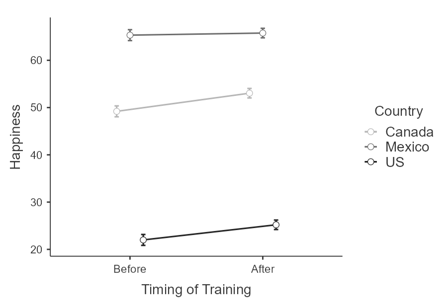
Note. Error bars represent 95% CI.
Perhaps the easiest thing to see in this figure is that there seem to be three bands, a lower, a mid-range, and an upper band. These correspond to the countries (our main effect). We can start with this description, but there is more to the story. Within two of the countries (US and Canada), we see an increase in happiness from before training to after training. This is not the case for Mexico. This change in the relationship between Timing of Training and Happiness across Countries is the interaction effect we detected in the ANOVA.
What about the main effect of timing of training? Although the marginal means (see figure 8) suggest a reliable increase in happiness ratings after training compared to before training, we should not report this because it is not true for all countries (see "Mexico" data in figure 7).
Figure 8
Main Effect of Timing of Training
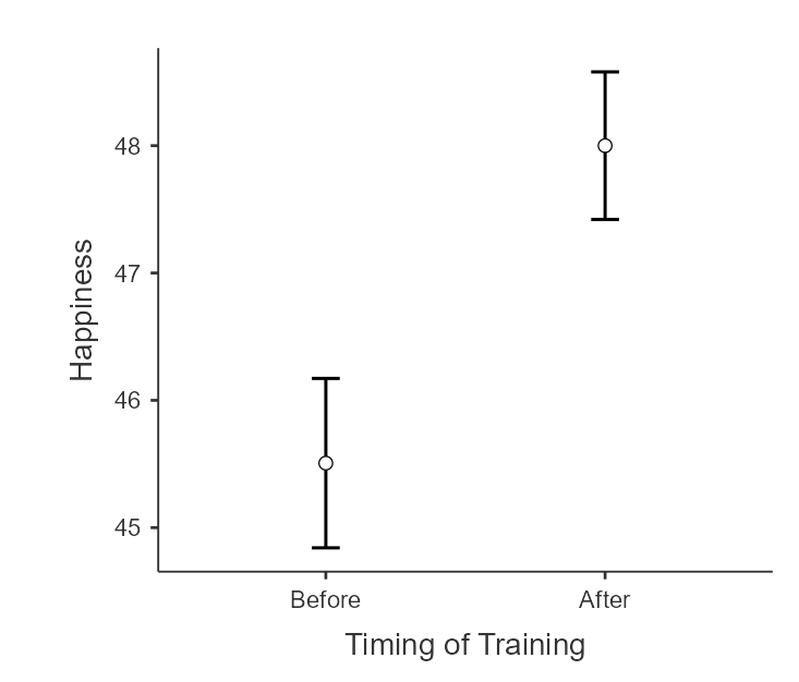
Note. Error bars represent 95% CI
I suggest including the estimated marginal means tables for the interaction (table 7) and for the main effect of country (table 8) for references in the write-up.
Table 7
Estimated Marginal Means for Interaction Effect
| Country | Timing of Training | Mean | SE | 95% CI Lower | 95% CI Upper |
|---|---|---|---|---|---|
| Canada | Before | 49.2 | 0.583 | 48.0 | 50.4 |
| After | 53.0 | 0.508 | 52.0 | 54.0 | |
| Mexico | Before | 65.3 | 0.583 | 64.2 | 66.5 |
| After | 65.8 | 0.508 | 64.8 | 66.8 | |
| US | Before | 22.0 | 0.583 | 20.8 | 23.2 |
| After | 25.2 | 0.508 | 24.2 | 26.2 |
Table 8
Estimated Marginal Means for Main Effect of Country
| Country | Mean | SE | 95% CI Lower | 95% CI Upper |
|---|---|---|---|---|
| Canada | 51.1 | 0.427 | 50.3 | 52.0 |
| Mexico | 65.5 | 0.427 | 64.7 | 66.4 |
| US | 23.6 | 0.427 | 22.8 | 24.4 |
The Write-Up
One last reminder to include the three components of each part of the write up:
- State the test
- Interpret the results
- Provide statistical evidence
To determine the impact of timing of mindfulness training and country of origin on happiness rating, I needed to perform a mixed factorial analysis of variance. The assumptions of this analysis are normality of the outcome variable values within each sample, homogeneity of variance, and sphericity. I test for normality by checking skewness and kurtosis values, which were all within 2 SE of 0 (see table 1). I checked the assumption of homogeneity of variance using Levene's test. These tests indicated no violation for happiness ratings before training (F[2,147] = 0.957, p = 0.386) but a violation for happiness ratings after training (F[2,147] = 4.625, p = 0.011). This violation is not a concern because the sample size is large and balanced (N = 150, n = 50 per country). The assumption of sphericity does not apply to this design because the within-subjects variable (i.e., timing of training) only has two levels (i.e., before and after).
The analysis of variance revealed a significant interaction effect (F[2,147] = 7.01, p = 0.001, η2p = 0.087) and significant main effects (FTiming [1,147] = 40.05, p < .001, η2p = 0.214; FCountry[2,147] = 2488, p < .001, η2p = 0.971). The interaction plot (see figure 1) reveals a main effect of country such that Mexico has highest happiness ratings, on average, followed by Canada and then by the U.S. (see table 2 for means and 95% CI). The interaction seems to be driven by the increase in happiness scores after training for the U.S. and Canada, but not for Mexico (see table 3 for pairwise comparisons and table 4 for means and 95% CI)
Table 1
Skewness and Kurtosis Values for Happiness Ratings by Timing of Training and Country
| Timing of Training | Country | Skewness | SE | Kurtosis | SE |
|---|---|---|---|---|---|
| Before | Canada | 0.496 | 0.337 | -0.0844 | 0.662 |
| Mexico | 0.208 | 0.337 | -1.0248 | 0.662 | |
| US | 0.661 | 0.337 | 0.1296 | 0.662 | |
| After | Canada | -0.487 | 0.337 | -0.5664 | 0.662 |
| Mexico | 0.440 | 0.337 | 0.0999 | 0.662 | |
| US | -0.630 | 0.337 | 0.2317 | 0.662 |
Figure 1
Interaction Plot of Timing of Training and Country on Happiness Ratings

Note. Error bars represent 95% CI.
Table 2
Estimated Marginal Means for Main Effect of Country
| Country | Mean | SE | 95% CI Lower | 95% CI Upper |
|---|---|---|---|---|
| Canada | 51.1 | 0.427 | 50.3 | 52.0 |
| Mexico | 65.5 | 0.427 | 64.7 | 66.4 |
| US | 23.6 | 0.427 | 22.8 | 24.4 |
Table 3
Bonferroni Post Hoc Comparisons of Before and After Training Happiness Ratings
| Country | Mean Difference | SE | df | t | pBonferroni |
|---|---|---|---|---|---|
| Canada | -3.840 | 0.682 | 147 | -5.627 | < .001 |
| Mexico | -0.440 | 0.682 | 147 | -0.645 | 1.000 |
| US | -3.200 | 0.682 | 147 | -4.689 | < .001 |
Note. Only within-country comparisons are shown
Table 4
Estimated Marginal Means for Interaction Effect
| Country | Timing of Training | Mean | SE | 95% CI Lower | 95% CI Upper |
|---|---|---|---|---|---|
| Canada | Before | 49.2 | 0.583 | 48.0 | 50.4 |
| After | 53.0 | 0.508 | 52.0 | 54.0 | |
| Mexico | Before | 65.3 | 0.583 | 64.2 | 66.5 |
| After | 65.8 | 0.508 | 64.8 | 66.8 | |
| US | Before | 22.0 | 0.583 | 20.8 | 23.2 |
| After | 25.2 | 0.508 | 24.2 | 26.2 |