The One-Way Between-Subjects ANOVA
The One-Way Between-Subjects ANOVARelevant Research QuestionsPost Hoc AnalysesAssumptionsNull HypothesisThe ANOVA Fraction and the F-distributionThe ANOVA TableThe Tukey HSD TableUsing jamovi for the One-Way Between-Subjects ANOVAThe Data SetThe Research QuestionChecking AssumptionsNormality of DV for Each GroupEqual Variance Across GroupsGenerating the ANOVAInterpreting ANOVA ResultsThe ANOVA TableTukey HSD TestsEstimated Marginal MeansWriting up the ANOVA resultsAssumption ChecksNormalityHomogeneity of Error VarianceANOVAPost HocCombined Write-upSummary
We are starting off with the simplest form of the ANOVA, the one-way between-subjects ANOVA. We outlined the “ANOVA” approach (i.e., dividing a distribution of scores into effect and error variances) in the previous section . We reviewed “between-subjects” designs (i.e., each participant receives only one level of the IV) when discussing the independent samples t-test. The new term to discuss is “one-way”. This refers to the number of independent variables/predictors in our design. As such, a “one-way between-subjects ANOVA” is a statistical analysis for determining the effect of one IV with levels administered to separate groups. A two-way ANOVA has two predictors and a seven-way ANOVA has seven predictors.
ANOVA, T-Test, and GLM
Traditionally, we would reserve the ANOVA for designs with more than 2 groups. With only two groups, a t-test is appropriate. However, because the ANOVA is more general than the t-test, it can be used in the same ways as the t-test. Furthermore, because the general linear model is more general than the ANOVA, it can handle ANOVA and t-test.
Relevant Research Questions
As the name suggests, we’d employ the one-way between-subjects ANOVA when we are interested in examining the effect of just one independent variable / predictor on a continuous dependent variable / outcome. The IV can have any number of levels but there are constraints. The more levels you have, however, the more data you need to detect differences.
Here are a few examples
- Does the type of breakfast influence alertness levels?
- Do the types of psychotherapy differently impact anxiety?
- Does the study technique used lead to differen test scores?
I’ve intentionally phrased these as yes/no questions rather than as “which” questions. This is because the ANOVA can only tell us if there is an effect of the IV, but does not tell us about specific patterns among the levels of the IV. That is, it can tell us that the means of the samples vary significantly (relative to sampling error) but it can not tell us which of the means are reliably different from other means.
If we were studying the effect of type of breakfast on alertness levels, we may ask some individuals to eat a balanced breakfast, some to eat a high protein breakfast, and another group to have a high carb breakfast. The ANOVA could tell us that the type of breaksfast does matter but would not reveal which is best or worst.
That may seem like the ANOVA is fairly pointless. It would be like telling the server at a restaurant that you are ready to order but not telling them what you want! The ANOVA is just the first step in a two-step process.
Post Hoc Analyses
The ANOVA can tell us if there is an effect. We need post hoc (i.e., “after the event”) tests to determine the pattern of the effects.
For the between-subjects one-way ANOVA, our post hoc test is the Tukey Honestly Signifacnt Difference (HSD) test. It is a modified version of the independent samples t-test we discussed in a previous lesson. The modification comes in the form of adjusting sampling distributions based on the number of comparisons being performed.
The order of procedures is important here:
- Check Assumptions
- Perform ANOVA
- Check for significant effect
- Perform post hoc test ONLY IF EFFECT IS SIGNIFICANT
jamovi update the output as we select options for our ANOVA so we can stop if the effect of our IV is not statistically significant. Of course, one could simply continue to add on to the output if they wanted. Regardless of how we generate the output (sequentially or in total), If we fail to reject the null hypothesis for the ANVOA but then claim that two of the means are reliably different, we are presenting conflicting information (and likely a false positive). Again, we can only report significant post hoc results IF AND ONLY IF we have a significant effect in the ANOVA.
Assumptions
For the conclusion of ANOVA to be valid, there are certain assumptions about the data that need met. These are the same as the independent samples t-test.
- Normally distributed dependent variable for each group. Since we are calculating means for each sample, we need to verify this assumption for each sample.
- Equal variance of dependent variable for each group. This assumption is also known as homogeneity of variance. When variances are unequal, our estimate of sampling error requires adjustment.
We will discuss how to check these assumptions using SPSS in the sections that follow.
Null Hypothesis
In the general form, the null hypothesis for ANOVA is the same as the t-test. That is, we start with the assumption that all of the samples are derived from the same population. That means we should expect that all the sample means are equal and thus equal to the population mean. We could state this general form as:
The null hypothesis, applied to research, is that we have no effect of an IV / predictor variable. To update our null hypothesis to the more specific version for ANOVA, we need to think about how our scores would vary, if there was no effect.
Although it is tempting to think that the variability would equal zero, we must still account for sampling error. That is, even without the influence of an IV, our scores will vary randomly around the population mean. As such, we should expect that our fraction (e.g.,
The ANOVA Fraction and the F-distribution
It is time to update our statistical test formula.
Notice that we’ve switched from calculating a t-value to an F-value. We have a new letter because we have a new sampling distribution. Whereas t-values could be positive or negative, F-values can only be positive because variances are squared values. This changes the shape of the distributions from normal to positively skewed and is determined by the degrees of freedom.
The ANOVA Table
You will find the degrees of freedom, F-values, p-values, and more for the different sources of variance in an Analysis of Variance (ANOVA) table. Table 1 is a prototypical ANOVA table.
Table 1
Prototypical ANOVA Table
| Source | Sum of Squares | df | Mean Square | F | p |
|---|---|---|---|---|---|
| Pet | 255.00 | 2 | 127.5 | 246.61 | .000 |
| Error | 15.00 | 27 | .517 | – | – |
| Total | 270.00 | 29 | – | – | – |
The row that starts with “Pet” is the “effect variance.” It contains the information related to the statistical significance of the independent variable. The “Error” row is related to the error variance. The “total” row is the combination of all the variances associated with factors and errors.
Interpretation of the table happens in two steps.
- Find the row for the effect your are interested in. If you have a one-way ANOVA, there will only be one that is labeled with your IV.
- Check if the p-value is less than α (i.e., .05)
If the p-value is less than α, we will reject the null hypothesis and claim that the IV has an effect on the DV. We would then move on to interpreting the post hoc tests (Tukey HSD in this case).
The Tukey HSD Table
In jamovi, the Tukey HSD results are presented in a table titled “Post Hoc Comparisons” because it presents the results of comparing each group to each other group. Figure 1 is an example from jamovi.
Figure 1
Example Post Hoc Comparison Table in jamovi

As with the ANOVA table, you’ll want to select the comparison of interest (e.g., Cat vs. Dog) then check if the “ptukey.” value is less than α.
If the p-value is less than α, we will reject the null hypothesis that the two samples came from the same population. It is possible (and likely more common than not) to have a significant ANOVA and some of the comparisons not reach statistical significance. Remember, ANOVA tells us that there is some effect, but does not reveal the pattern.
The “Post Hoc Comparisons” table focuses on the difference of the groups so it does not report the means of each group. You can get the means, standard deviations, and 95% Confidence Intervals from the “Estimated Marginal Means” table.
Using jamovi for the One-Way Between-Subjects ANOVA
I like jamovi for several reasons but the reason I think students will like jamovi is the ease of conducting analyses by selecting options in an easy-to-navigate interface. We'll walk through the one-way between-subjects ANOVA, step-by-step, to ensure you see all the options in order.
The Data Set
I'll be using the TeachingExample.omv dataset that I used in the Descriptive Statistics post. Because of the similarity in the structures of the datasets, you can follow along with the dataset you were provided.
The Research Question
For this post, we'll try to answer the following: "Does one's country of origin impact average happiness rating after receiving mindfulness training?"
The one-way between-subjects ANOVA seems appropriate for this question and data set because we have an IV with more than two groups (country has three levels: Canada, USA, and Mexico) and a continuous DV. We’ll need to check our assumptions regarding normality and homogeneity of variance to be sure it is appropriate, however.
Checking Assumptions
Normality of DV for Each Group
The assumption of normality needs to hold because we will be calculating means in determining if there is a reliable difference between the groups.
We'll be checking this assumption by looking at the skewness and kurtosis statistics for severe deviations form normality., We will then match these statistics with our interpretation of the Q-Q plots
Go to the "Analyses" tab and click the "Exploration" option (see figure2 )
Figure 2
Exploration Menu under Analyses Tab

Next, drag one of your marginal outcome values (i.e., one of the averaged outcome values) to the "Variables" box. In my example, I'm using the last one in my list of variables: "Happiness_After". Remember which you choose because that will be the same outcome variable you will use in the ANOVA. Now choose the between-subjects variable that has three levels. In my example, that is "Country". Drag that variable to the "Split by" box. This set up will allow us to examine each sample of "Happiness_After" ratings for each country of origin. Lastly, reorient your tables by selecting "Variables across rows" next to the "Descriptives" label. Figure 3 contains the setup of the variables.
Figure 3
Variables for Descriptive Statistics

With our variables set, it's time to tell jamovi what we want to see. In the "Statistics" section, choose "Skewness" and "Kurtosis" under the "Distribution" label. You can unselect all the other options. See figure 4 for the setup of the "Statistics" section.
Figure 4
Skewness and Kurtosis Options

To help us better understand what these values represent, we'll want jamovi to generate Q-Q plots, too. Go to the "Plots" section and turn on the "Q-Q" option under the "Q-Q Plots" label (see Figure 5).
Figure 5
Q-Q Plots Option

As we've added options, jamovi has been updating the output area. Let's review the skewness and kurtosis values and the Q-Q plots. I'll be referencing my output but yours may look a little different. That's okay. I'll remind you of the guiding principles as we go. Let's start with skewness and kurtosis (see table 2)
Table 2
Skewness and Kurtosis Values
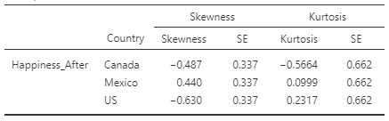
Recall that the skewness statistic is a quantification for asymmetry. Typically, a positive value indicates a longer tail on the right of the distribution (larger values are more extreme than smaller values) and a negative value indicates a longer tail on the left (smaller values are more extreme than larger). How asymmetrical is too asymmetrical? Generally speaking, as long as our skewness values are not more than twice the size of the SE value, we can continue with our assumption of normality. ANOVA happens to be particularly robust against violations of normality so skewness values up to 3 times the SE will only slightly impact the type I error rate.
Kurtosis is a measure of how thin or thick the tails of the distribution are, relative to a normal distribution. ANOVA is fairly insensitive to kurtotic distributions (up to 8 standard errors) so we are well within the bounds of acceptability with the values in Table 2 (largest is 0.85 standard errors).
Acceptable Skewness and Kurtosis Values
Skewness and kurtosis values that are less than twice the associated standard error are considered indicative of an acceptable normal distribtuion.
Kurtosis values can range up to 8 standard errors and skewness can range up to 3 standard errors before impacting conclusions form the ANOVA
Let's compare these interpretations to the Q-Q plot we produced (see Figure 6)
Figure 6
Q-Q Plots of DV by IV levels

These plots look "OK". Not perfect but good enough as the majority of the points lie along the normal reference line. As we saw in table 2, we do have some slight skewness (some bowing in the middle) and some kurtosis (deviation at the ends) but they are within acceptable ranges.
Equal Variance Across Groups
The other assumption we need to verify is that we have equal variance across groups. We’ll ask jamovi to perform Levene’s Test for Equality of Variances when we generate the ANOVA. Levene's test constructs a ratio, much like we do in an ANOVA to determine if the the variances in groups are more different than expected by chance. jamovi will provide us an F-value and p-value for Levene's test and we can interpret that as any F-value and p-value.
However, just as with our normality checks, we have more to consider than one cut-off (i.e., when p-value is less than α, or .05). If we have a significant Levene's test (i.e., suggesting a violation of the assumption of the equality of error variances), we need not panic.
- If your samples sizes are equal, don't sweat this at all as unequal variances are inconsequential.
- If you sample sizes are unequal but greater than 50, Levene's test can be overly sensitive for larger sample sizes and indicate a violation when the differences in variance are slight. Check the variances for each sample and if the largest is less than nine times the smallest, the impact should be minimal.
- If your samples sizes are small (< 50) and your variances are unequal, you should pay attention to the result of Levene's test. When there is a violation, you should use a non-parametric alternative (e.g., Kruskal-Wallis) and compare results with your ANVOA.
We'll check on Levene's test after we get our ANOVA set up
Generating the ANOVA
ANOVA has its own menu under the "Analyses" tab (see figure 7).
Figure 7
ANOVA Menu under Analyses Tab

The first section of the ANOVA panel is very similar to the Descriptives panel: our outcome variable goes in the first box ("Dependent Variable") and our predictor variable goes in the second box ("Fixed Factors"). In this example, the outcome variable is "Happiness_After" and the predictor variable is "Country." We'll want to include a measure of effect size with to get a better sense of the impact of our predictor on our outcome, beyond being "statistically significant." Choose the first option under the "Effect Size" label (η2 pronounced eta-squared ["Eh-tuh" squared]). This value represent the proportion of variance in the outcome variable that is accounted for by the predictor variable. Essentially, the larger (up to 1) the value, the stronger the predictor. See figure 8 for the complete variable section setup.
Figure 8
Variable Placement in ANOVA Setup

The next section we'll need to visit is the "Assumption Checks" section. In this area, please turn on the "homogeneity test" option to run "Levene's test". "Normality test" and "Q-Q Plot" are options here but we've already checked our assumption of normality before starting the ANOVA (see Figure 9).
Figure 9
Assumption Check Options in ANOVA

Should we have a statistically significant impact of our predictor ("Country") on our outcome ("Happiness_After") variable, we'll need to follow-up with a post-hoc test to determine which countries of origin have reliably different happiness scores after mindfulness training. Remember, ANOVA can only tell us IF a reliable difference exists but it cannot tell us between which groups that difference exists. Drag our predictor variable from the box on the left to the box on the right. We'll investigate any group-level differences using the Tukey test and we'll also ask for a measure of effect size ("Cohen's D"). Figure 10 shows the "Post Hoc Tests" panel after setup.
Figure 10
Post Hoc Tests Options in ANOVA

The last section we need to update is the "Estimated Marginal Means" section. This will give us information about the calculated means for each sample and the range of values we might expect from other samples. Drag the predictor variable from the box on the left to the "Marginal Means" box on the right, under "Term 1." You will also need to turn on the options for "Marginal means tables" (see figure 11)
Figure 11
Estimated Marginal Means Options in ANOVA

As you've likely noticed, jamovi has been updating the results section on the right side of the window. Let's walk through those next.
Interpreting ANOVA Results
Before we get to the ANOVA itself, we need to check on our last assumption, equality of error variances. Let's look at Levene's Test which is depicted in table 3.
Table 3
Levene's Test

This test has a p-value of .011, which is less than α = .05. This means that Levene's test is indicating a violation of the assumption of equality of error variances. However, before we abandon this ANOVA, let's remember that we have equal sample sizes. Furthermore a check of sample variances (see table 4) indicates that the largest variance (Mexico) is only 2.18 times greater than the smallest (Canada). As such, even if we did not have equal sample size, this suggests that our results would not be impactfully altered.
Table 4
Sample Variances

To summarize our assumption checks, we find that we have not severely violated normality (skewness and kurtosis within range) or equality of variance for this one-way between-subjects ANOVA.
The ANOVA Table
We can proceed to the ANOVA table (see Table 5) to determine if we have a reliable impact of our predictor variable on our outcome variable.
Table 5
ANOVA Table

The results of the stable indicate that there is a statistically significant effect of "Country" on "Happiness_After" with a p-value < .001. The effect size (η2) also suggests that the effect is sizeable by accounting for over 95% of the variability in the outcome variable. Again, this tells us that we have some difference in happiness ratings after mindfulness training due to a participant's country of origin but it does not tell us which countries are different in happiness ratings. We'll have to move on to the estimated marginal means and post hoc tests for that.
Tukey HSD Tests
The Tukey HSD Tests are presented in table 6. Tukey's HSD is essentially an adjusted t-test (controlling for multiple comparisons) so we'll interpret it the same way, if the p-value is less than α, we will reject the null hypothesis that the samples are derived from the same population. Table 6 also shows another measure of effect size, Cohen's d. Table 7 has some key values and interpretations for Cohen's d.
Table 6
Tukey HSD Tests Results

First we should notice that the pTukey values are all <.001, which indicates that the differences between the groups are not due to chance alone. The Cohen's d values are also telling. Each are in the "Huge" category.
Table 7
Key Values for Cohen's d
| d | Effect size |
|---|---|
| 0.01 | Very small |
| 0.20 | Small |
| 0.50 | Medium |
| 0.80 | Large |
| 1.20 | Very large |
| 2.0 | Huge |
These results are encouraging but they aren't easy to communicate to others. It is helpful to present the data in the original metrics. Let's reference the estimated marginal means to see the average happiness ratings for each country.
Estimated Marginal Means
The estimated marginal means provide the mean of the samples but helps one extend to what may be found in other samples of the same size with confidence intervals. Table 8 contains the marginal means and 95% confidence intervals (CI) for each country.
Confidence Intervals contain the lowest expect and the highest expect value to occur in same-sized samples, with a certain level of confidence. The confidence level is calculated as 1 - α. As such, the most common confidence intervals are at 95% because α is typically set to .05.
Table 8
Estimated Marginal Means Table

To reinforce the connections across analyses, you can reach the same conclusion as the Tukey HSD tests using these 95% CI for each country. If the 95% CI do not overlap, there is less than a 5% chance that the samples will have the same mean. That is, we would reject the null hypothesis at α = .05 when two 95% CI have no overlap (i.e., the lower bound of one interval is greater than the upper bound of the other). This is certainly the case for these means, but this takes some cognitive effort. A figure makes these differences even more apparent. Figure 12 is an error bar plot of the estimated marginal means and 95% CI error bars
Figure 12
Estimated Marginal Means Error Bar Plot

In this error bar plot, the circles are plotted on the sample mean and the error bars represent the 95% CI around the mean. Again, we see no overlap in these ranges.
Now that we've reviewed all the output, it is time to put the results in a presentable format.
Writing up the ANOVA results
Sharing the results of statistical analyses follows a pattern:
- State the test
- Interpret the results of the test
- Provide statistical evidence for the interpretation
Stated another way, you should answer the following questions for each analysis:
- What did you do?
- What did you find?
- What makes you think that?
I wrote that this should be applied to every analysis and this includes assumption checks and post-hoc comparisons. The full outline of our write-up for an ANOVA is:
Assumption checks
- State the test
- Interpret the results of the test
- Provide statistical evidence for the interpretation
ANOVA
- State the test
- Interpret the results of the test
- Provide statistical evidence for the interpretation
Post-hoc
- State the test
- Interpret the results of the test
- Provide statistical evidence for the interpretation
Our write-up is more than a presentation of facts because Statistics is ultimately a collection of decision-guiding tools. This makes our write-up a persuasive argument, although it is not often framed as such. Essentially, we would like our readers to agree with our conclusions and we'll need to provide them with all the necessary information to come to that decision. Let's walk through the full process and then put it all together.
Assumption Checks
Normality
State the Test
The one-way between-subjects ANOVA assumes normally distributed values in the population and equal error variance across samples. I checked the assumption of normality by calculating skewness and kurtosis statistics.
Interpret the Results
The skewness and kurtosis statistics indicated normal distributions.
Provide Statistical Evidence
All values were within 2 standard errors (see table 1)
Homogeneity of Error Variance
State the Test
I checked the assumption of homogeneity of error variance with Levene's test.
Interpret the Results
Levene's test indicated a violation of the assumption but this is not much of a concern as the sample sizes are equal and the largest ratio of variances across groups was 2.18.
Provide Statistical Evidence
Levene's test resulted in F(2,147) = 4.63, p = .011, but each sample had n = 150 and the samples variances were not drastically different (varianceCanada = 8.20, varianceMexico = 17.90, varianceUS = 12.57).
F-test Write-up
When presenting the results of an F-test in a write-up, it should follow this format:
F(dfeffect,dferror) = F-value, p = p-value
Note. if the p-value is less than .001, you can write "p < .001", otherwise, write the actual p-value.
ANOVA
State the Test
To determine the impact of country of origin on happiness rating after mindfulness training, I performed a one-way between-subjects ANOVA using jamovi.
Interpret the Results
The ANOVA indicated an reliable impact of country on happiness.
Provide Statistical Evidence
The ANOVA yielded F(2,147) = 1669, p < .001, η2 = .958.
Post Hoc
State the Test
To determine which countries have different happiness ratings after mindfulness training, I used Tukey HSD tests.
Interpret the Results
All comparisons were statistically significant.
Provide Statistical Evidence
Table 2 contains the results of Tukey HSD comparisons and associated effect sizes. Mexico reported the highest levels of happiness ratings (M = 65.8, 95% CI [64.8, 66.8]), followed by Canada (M = 53.0, 95% CI [ 52.0, 54.0]), and the U.S. reported the lowest levels (M = 25.2, 95% CI [24.2,26.2]). See figure 1 for corresponding error bar chart.
Great! We now have all the pieces that we can put together into one cohesive write-up.
Combined Write-up
The one-way between-subjects ANOVA assumes normally distributed values in the population and equal error variance across samples. I checked the assumption of normality by calculating skewness and kurtosis statistics. The skewness and kurtosis statistics indicated normal distributions. All values were within 2 standard errors (see table 1). I checked the assumption of homogeneity of error variance with Levene's test. Levene's test indicated a violation of the assumption (F[2,147] = 4.63, p = .011) but this is not much of a concern as the sample sizes are equal (n = 150) and the largest ratio of variances across groups was 2.18 (varianceCanada = 8.20, varianceMexico = 17.90, varianceUS = 12.57). To determine the impact of country of origin on happiness rating after mindfulness training, I performed a one-way between-subjects ANOVA using jamovi. The ANOVA indicated an reliable impact of country on happiness (F[2,147] = 1669, p < .001, η2 = .958). To determine which countries have different happiness ratings after mindfulness training, I used Tukey HSD tests. All comparisons were statistically significant. Table 2 contains the results of Tukey HSD comparisons and associated effect sizes. Mexico reported the highest levels of happiness ratings (M = 65.8, 95% CI [64.8, 66.8]), followed by Canada (M = 53.0, 95% CI [ 52.0, 54.0]), and the U.S. reported the lowest levels (M = 25.2, 95% CI [24.2,26.2]). See figure 1 for corresponding error bar chart.
Table 1
Skewness and Kurtosis Values
Table 2
Tukey HSD Results
Figure 1
Marginal Mean Error Bar Chart
Summary
In this post, we:
- Stated the relevent research questions for one-way between-subjects ANOVA,
- Explored the assumptions of the one-way between-subjects ANOVA,
- Described the need for post hoc analyses,
- Checked the assumptions of ANOVA in jamovi,
- Set up and run an ANOVA in jamovi,
- Conducted post hoc tests in jamovi,
- Interpreted the results of the anova, and
- Shared the results in APA format.
In the next lesson, we’ll examine the the generalized version of the paired samples t-test: the within-subjects ANOVA.