The Within-Subjects ANOVA
The Within-Subjects ANOVAResearch Designs for the Within-Subjects ANOVAThe Null HypothesisThe FormulaComparing Within-Subjects ANOVA with Between-Subjects ANOVAPartitioning Error FurtherIncreased Statistical PowerPost Hoc AnalysesAssumptionsUsing jamovi for the One-Way Within-Subjects ANOVAThe Data SetThe Research QuestionChecking AssumptionsNormality of DV for Each SampleSphericity: Equal variance across differencesGenerating the ANOVATop Panel (Variable Assignment)Assumption ChecksPost Hoc TestsEstimated Marginal MeansInterpreting the ANOVA ResultsMauchly's Test of SphericityThe ANOVA TableBonferroni TestsEstimated Marginal MeansWriting up the ANOVA resultsRevisiting the FormatThe Write-UpSummary
The within-subjects analysis of variance (ANVOA) is the generalization of the paired-samples t-test. That is because it is used when we have repeated measures of a dependent variable but with more than two levels of an independent variable. To account for the increased number of samples, we will need to take the analysis of variance approach. We’ll find, however, that there are some important changes from the between-subjects ANOVA
Repeated measures refers to designs in which one or more dependent variables are measured multiple times from each participant.
Research Designs for the Within-Subjects ANOVA
Recall that a within-subjects design requires each participant to experience all levels of an independent variable. That means that each participant will have the same number of dependent variable measurements as there are levels of the independent variable.
One of the classic designs of this style is called the longitudinal design. In this approach, a researcher may be interested in how outcome variables may change as a factor of time. Some examples include cognitive development, political ideation, and language abilities.
Longitudinal designs are those in which outcome variables are assessed over time, often at regular intervals.
In a more experimental setting, a researcher might employ a “pre-post” design. These designs assess participants on the dependent variables before and after administering the levels of the independent variable. For example, a researcher who is interested in the effect of team building exercises might assess team cohesiveness before and after each of three different exercises (i.e., group problem solving, trust exercises, and shared recreation).
The key aspect of these designs is the ability to assess the change in the outcome variable related to the independent variable for each participant. Given that we are focusing on the differences within each individual, we’ll be able to hone our analysis and gain statistical power.
The Null Hypothesis
Just as with the one-way between-subjects ANOVA, the null hypothesis is that there is no effect of the IV causing our DV scores to vary; only sampling error. Because we are focusing on the difference scores, we would expect the mean of each of our comparisons to be equal
The Formula
We will utilize the same basic F-statistic for the within-subjects ANOVA
However, we’ll need to have to define “Effect” and “Error” slightly differently.
Comparing Within-Subjects ANOVA with Between-Subjects ANOVA
To understand how the within-subjects ANOVA differs from the between-subjects ANOVA, let’s build an example. We’ll imagine that we ask a group of job-seekers to each try one of three different social cuing techniques during interviews. On one interview, the job-seekers are asked to sit back in their chairs, looking relaxed. On another interview, they are asked to sit on the edge of their chairs, looking eager. On a third interview, we ask them to sit upright but fully in the chair for the control condition. After each interview, we ask the interviewer to rate the job-seeker on employability.
The employability ratings for each job-seeker in each interview is presented in table 1.
Table 1
Job-Seeker Employability Ratings across Social Cuing Conditions
| Job-Seeker | Control | Relaxed | Eager |
|---|---|---|---|
| A | 4 | 2 | 9 |
| B | 6 | 3 | 8 |
| C | 5 | 1 | 7 |
Before we add in our marginal means, we need to calculate the differences among the conditions for each participant. Table 2 contains the differences of ratings among all combinations of levels of the social cuing.
Table 2
Differences in Job-Seeker Employability Ratings across Social Cuing Conditions
| Job-Seeker | Control - Relaxed | Control - Eager | Relaxed - Eager |
|---|---|---|---|
| A | 2 | -5 | -7 |
| B | 3 | -5 | -5 |
| C | 4 | -2 | -6 |
Now we can add in the marginal means to the bottom of the table. Table 3 contains the marginal means for each comparison of social cuing.
Table 3
Differences in Job-Seeker Employability with Marginal Means
| Job-Seeker | Control - Relaxed | Control - Eager | Relaxed - Eager |
|---|---|---|---|
| A | 2 | -5 | -7 |
| B | 3 | -5 | -5 |
| C | 4 | -2 | -6 |
| Marginal Means | 3 | -3 | -6 |
We can actually add another set of marginal means because we have an additional grouping factor in our design; job-seeker! However, we wouldn’t consider job-seeker to be an independent variable or predictor variable because we are concerned about the impact of individual job-seekers on employability ratings. However, it is something that varies systematically in our study and thuse can be utilized in the analysis. Table 4 contains the marginal means for job-seeker as well as for social cuing conditions.
Table 4
Differences in Job-Seeker Employability with All Marginal Means
| Job-Seeker | Control - Relaxed | Control - Eager | Relaxed - Eager | Marginal Means |
|---|---|---|---|---|
| A | 2 | -5 | -7 | -3.33 |
| B | 3 | -5 | -5 | -1.33 |
| C | 4 | -2 | -6 | -1.33 |
| Marginal Means | 3 | -3 | -6 | GM = -2 |
Let’s discuss how we can use these various marginal means in the ANOVA approach.
Partitioning Error Further
Recall that the ANOVA approach accounts for the factors that are causing our individuals scores to differ from the overall average (i.e., the grand mean). Table 4 emphasizes that we have two factors in a one-way within-subjects ANOVA; the independent variable and participant. Remember that the term “one-way” refers to the number of independent variables in our analysis and participant is not an independent variable.
Let’s revisit our ANOVA fraction from the one-way between-subjects ANOVA lesson.
Essentially, we are looking to compare the differences in the scores due to our independent variable to the differences in our scores due to random error (i.e., sampling error). We can easily use the variance due to social cuing (i.e., the variability of marginal means for the columns) as the numerator.
Where do we put the variability due to participant? Nowhere. We are actually going to remove it from the denominator (i.e., VarianceError). As such, our new ANOVA fraction for the within-subjects ANOVA becomes
When we subtract from the denominator, we are making the denominator smaller and thus making the overall fraction larger. This has implications for statistical power.
Increased Statistical Power
Statistical power refers to the probability of a test to detect an effect if it is actually there. The within-subjects ANVOA is statistically more powerful than the between-subjects ANOVA for any given sample size because of the way it eliminates the between-subjects variability from the error term. Given the same number of participants, we will be better able to detect a difference across conditions using a within-subjects design than a between-subjects design.
Of course, there are other things to consider than statistical power. For example, our job-seekers interviewing ability using one social cuing technique may be influenced by those used in previous interviews. These carry-over effects can be serious flaws in a study. There are ways to appropriately handle these issues but it comes at the cost of complicating the design.
Carry-over effects refers to the impact of previous trials on future trials.
Post Hoc Analyses
If (and I DO MEAN IF) we have a statistically significant F-test for the within-subjects ANOVA, we will need post hoc analyses. This is because the ANOVA only tells us that there is a difference across our IV levels but does not reveal which levels are different from other levels.
The post hoc analysis of choice for the within-subjects ANOVA is the Bonferroni-corrected paired samples t-test. The Bonferroni correction is a simple technique used to adjust for the increase Type I Error (i.e., false positive rate) incured with multiple tests. You simply divide your αα-level by the number of pairwise comparisons made.
The Bonferroni correction adjusts for increased Type I Error by dividing α by the number of tests.
In our example, we will have to perform three paired samples t-tests to compare all groups. The Bonferroni correction thus yields a new, adjusted α-level of
Assumptions
We are introducing a new assumption for the within-subjects ANVOA because of the extra step of calculating difference scores. It is analogous, however, to the assumption of equal variance.
- Sphericity. Sphericity refers to an equality of variance among the difference scores calculated in comparing each condition to each other condition.
- Normality. As we are calculating the means of the difference scores, we’ll want to ensure that they are normally distributed.
Using jamovi for the One-Way Within-Subjects ANOVA
You should find a lot of similarity in jamovi for completing these analyses as you had for one-way between-subjects ANOVA and that is a good thing. I'll point out the differences as we go walk through the full process.
The Data Set
I'm continuing with the TeachingExample.omv data set and you should follow along with your data set that was provided for the semester. As we work with the within-subjects data in this example, we'll have to pay attention to what is contained in each variable. These data sets are in the "wide format", which means there is no variable that contains the name and the levels for within-subjects variables like we had for between-subjects variables. Instead, the levels of the within-subjects variable are spread across columns (one column per level). That is, each within-subjects variable level is its own variable in jamovi. The values contained in those variables are the outcome variable values (happiness rating, in my example). Perhaps the trickiest part of this setup is that the within-subject variable name is not presented. You need to infer the within-subject variable from the level. Figure 1 presents the within-subjects related variables from jamovi. The figure has been annotated to include the within-subjects variables names.
Figure 1
Within-Subjects Variables in jamovi

The Research Question
For this one-way within-subjects ANOVA example, I want to use the within-subjects predictor variable that has three levels. In my data, this is the "time of day" variable. The research question I hope to answer, therefore, is "which time of day had the highest happiness ratings?"
Checking Assumptions
Assumption checking will be very similar to what we did for the one-way between-subjects ANOVA with one small change. Whereas we had to split out data according to our between-subjects variable to examine the samples, the wide-format data set already has the samples separated according to the within-subjects levels.
Normality of DV for Each Sample
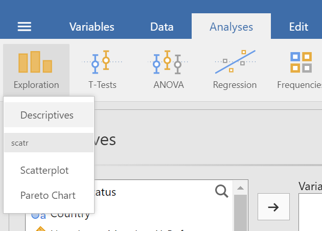
We can check for the normality of our samples by calculating skewness and kurtosis statistics as well as examining Q-Q plots. Click on the the "Exploration" menu button in the "Analyses" tab, then choose "Descriptives" (see figure 2).
Figure 2
Descriptives in Exploration Menu under Analysis Tab
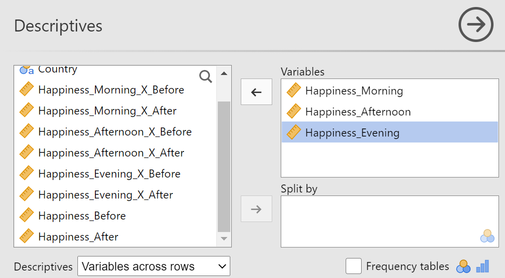
In the "Descriptives" top panel, drag the three variables that correspond to the three levels of your within-subjects variable (hint: they should be number 9, 10, and 11 in your list). Choose "Variable across rows" in the drop down list next to the "descriptives" label. Figure 3 shows the "Descriptives" top panel after setup.
Figure 3
Descriptives Top Panel after Setup
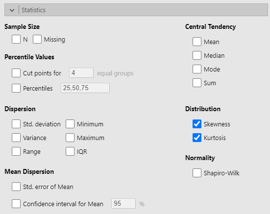
In the "Statistics" section, we need "Skewness" and "Kurtosis" from the "Distribution" area. I turned off all the other options to make my table easier to read, should I want to include it as evidence in my assumption check section of my write-up. Figure 4 represents the "Statistics" section.
Figure 4
Statistics Section of Descriptives Panel
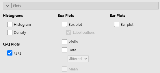
Last step is to turn on the "Q-Q" option under "Q-Q Plots" in the "Plots" section (see figure 5).
Figure 5
Q-Q Plots Option in Plots Section
With our output generated, we can come to some decisions about the distributions of our samples. Table 5 contains the skewness and kurtosis values and figure 6 contains the Q-Q plots.
Table 5
Skewness and Kurtosis Values of Within-Subjects Samples

Remember that skewness values that are less than 2x the corresponding standard error (SE) are within acceptable ranges and kurtosis values within 3x the corresponding SE are acceptable. The skewness values all check out but the kurtosis values are over 3 SE. Let's take a peak at the Q-Q plots for more information on the kurtosis.
Figure 6
Q-Q Plots of Within-Subjects Samples
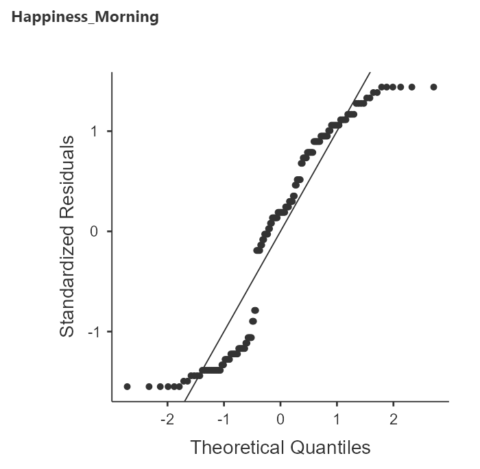
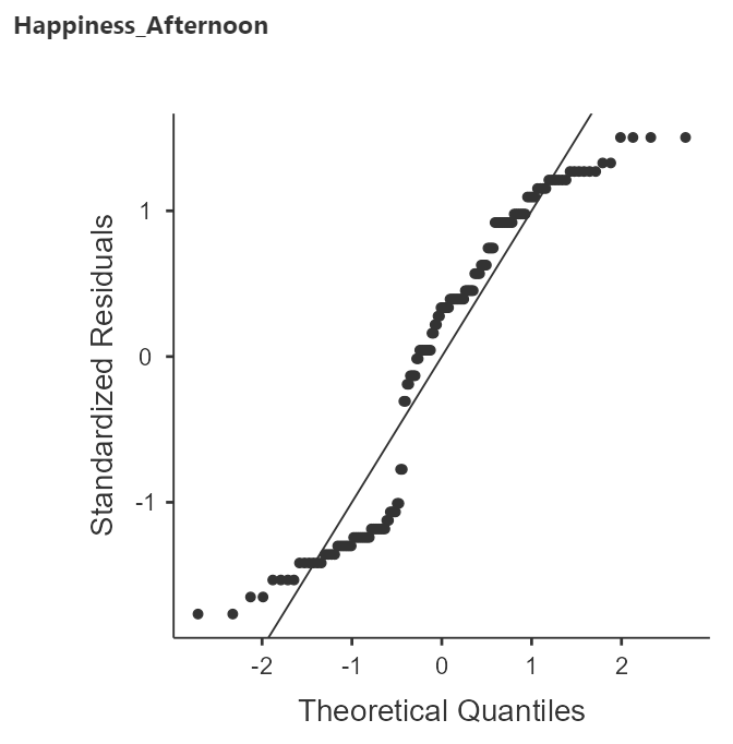
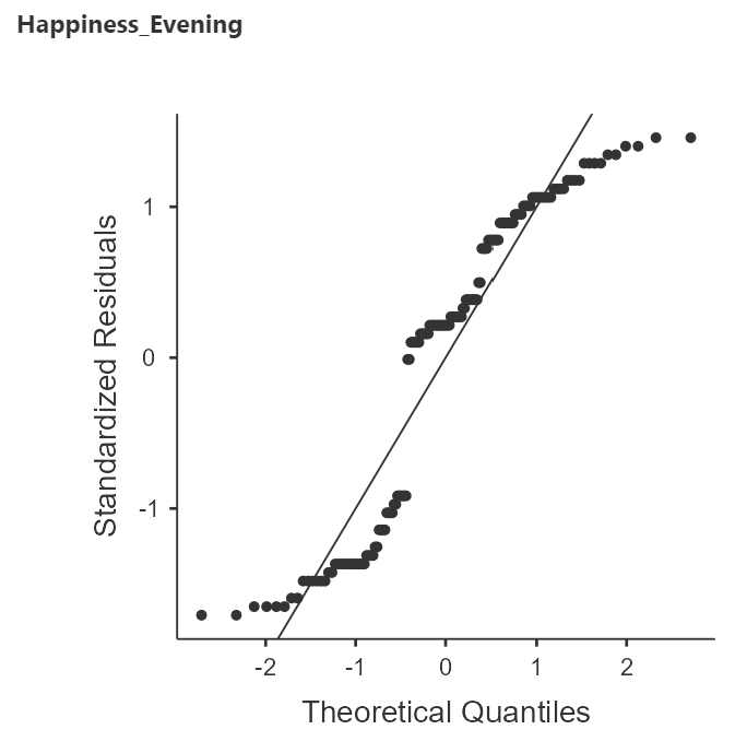
There is definitely some snaking happening in these plots but the kurtosis does not seem so extreme as to prevent us from continuing with the ANVOA.
Sphericity: Equal variance across differences
Just like the homogeneity in the between-subjects ANOVA, we'll ask for this when set up the ANOVA. Sphericity is tested with Mauchly's test of sphericity that produces a "W" statistic and a p-value. It will also give us some estimates for adjustments needed due to deviations from sphericity. If we have a violation (i.e., the p-value is less than α), we can use one of the adjustments provided (Greenhouse-Geisser or Huynh-Feldt). Generally, the Greenhouse-Geisser adjustment is the best option and we can ask jamovi to include this when we set up the ANOVA. These adjustments reduce the degrees of freedom as a sort of "penalty," making it more difficult to reject the null hypothesis.
Generating the ANOVA
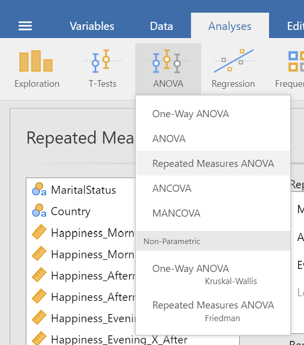
We need to get back into the "ANOVA" menu under the "Analyses" tab but this time we are selecting the "Repeated Measures ANOVA" option (see figure 7).
Figure 7
Repeated Measures ANOVA Option in ANOVA Menu under Analyses Tab
Top Panel (Variable Assignment)
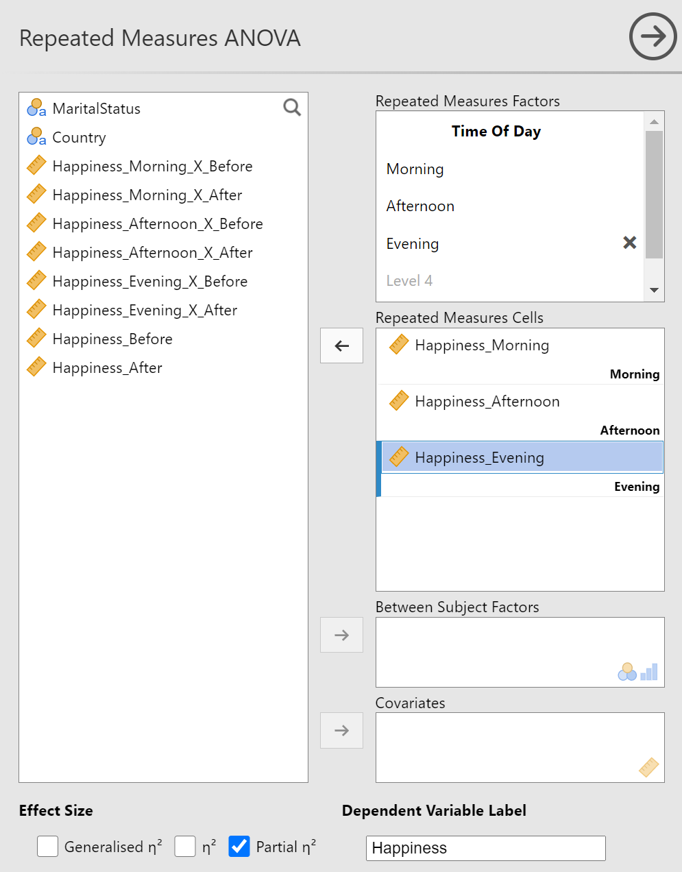
The "Repeated Measures ANOVA" panel is similar to the "ANOVA" panel we saw in the between-subjects ANOVA post but there are some important differences. Please refer to figure 8 as I describe each of the boxes.
Figure 8
Repeated Measures ANOVA Panel
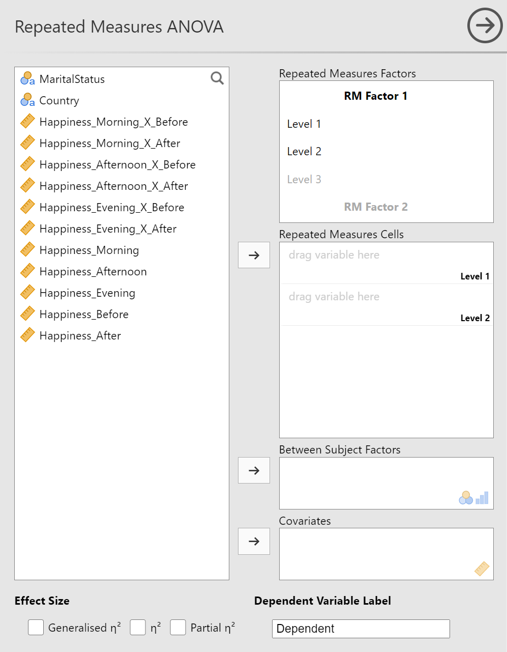
The familiar list of variables is on the left-hand side. You will move the variables from the left to different boxes on the right, depending on the model you're testing. We will be setting up a one-way within-subjects ANOVA so we'll just be using the first two boxes on the right.
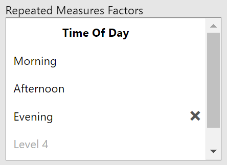
The "Repeated Measures Factors" box requires you to give names to your within-subjects variable and the levels. jamovi needs this information because it is not included in the dataset in the same way that it is for between-subjects factors. Click on "RM Factor 1" to activate the text box. Give it the name of your within-subjects variable that has three levels. In my example, that is "Time of Day". Next, click on "Level 1" and replace the text with the first level of your within-subjects variable. Mine will be "Morning". Continue this with "Level 2" and "Level 3". Figure 9 has my completed "Repeated Measures Factors" box.
Figure 9
Completed Repeated Measures Factors Box
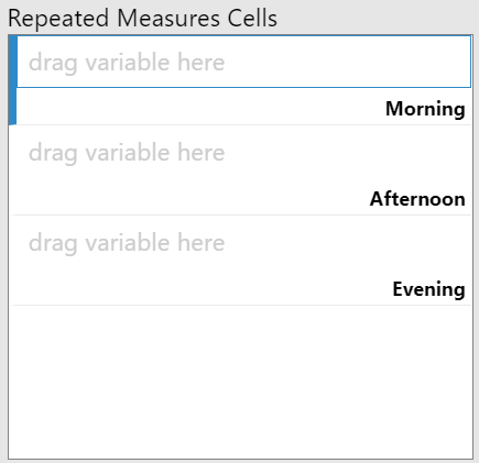
The next box, "Repeated Measures Cells" is where you'll align the variables that contain the outcome variable for each level of your within-subjects variable. As you can see in figure 10, jamovi has created a box for each of the levels you specified in the "Repeated Measures Factors" box.
Figure 10
Spaces for Variables in Repeated Measures ANOVA
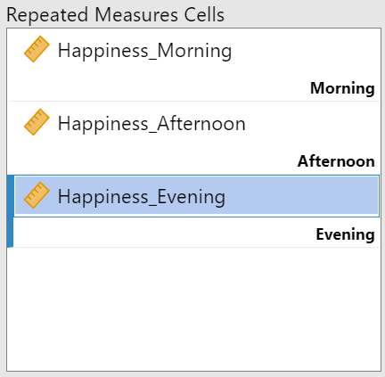
Luckily for us, it will be easy to know which variable goes where because our variables have labels that match the levels. Remember, you'll be using the same variables that you examined for the assumption of normality. Drag each variable to its corresponding space in the "Repeated Measures Cells" box. Figure 11 shows the completed alignment for my example.
Figure 11
Completed Repeated Measures Cells Box
The last description we'll need to provide jamovi about our data set is the "Dependent Variable Label," located at the bottom-right of the top panel. You should type in the name that is the first word of all your within-subject variable labels. In my example, it is "Happiness."
While you're in the vicinity, check the "Partial η2" option in the "Effect Sizes" area. That's it for this section. You can see the completed panel in figure 12.
Figure 12
Completed Top Panel of Repeated Measures ANOVA Setup
Assumption Checks
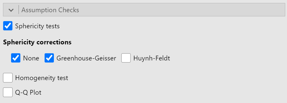
Move to the "Assumption Checks" section and activate the "Sphericity tests" options. Then check the "None" and "Greenhouse-Geiser" options under "Sphericity corrections". We do not need to include "Homogeneity test" because this is for models that include between-subjects variables. See figure 13 for the completed "Assumption Checks" section.
Figure 13
Completed Assumption Checks Section
Post Hoc Tests
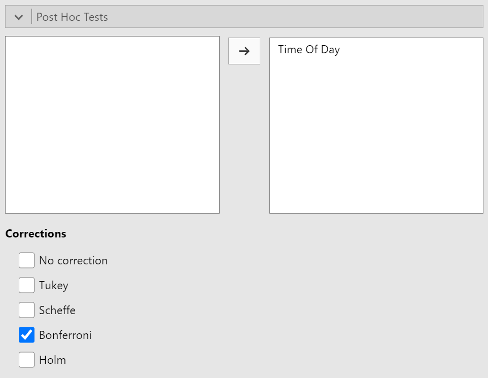
Move to the next section, "Post Hoc Tests." There are two steps for this section. First, you'll want to move your within-subjects variable from the area on the left to the area on the right. After that, choose the "Bonferroni" correction. Although this is a conservative correction, it is appropriate for the higher-powered within-subjects design. Figure 14 shows the completed "Post Hoc Tests" section
Figure 14
Completed Post Hoc Tests Section
Estimated Marginal Means
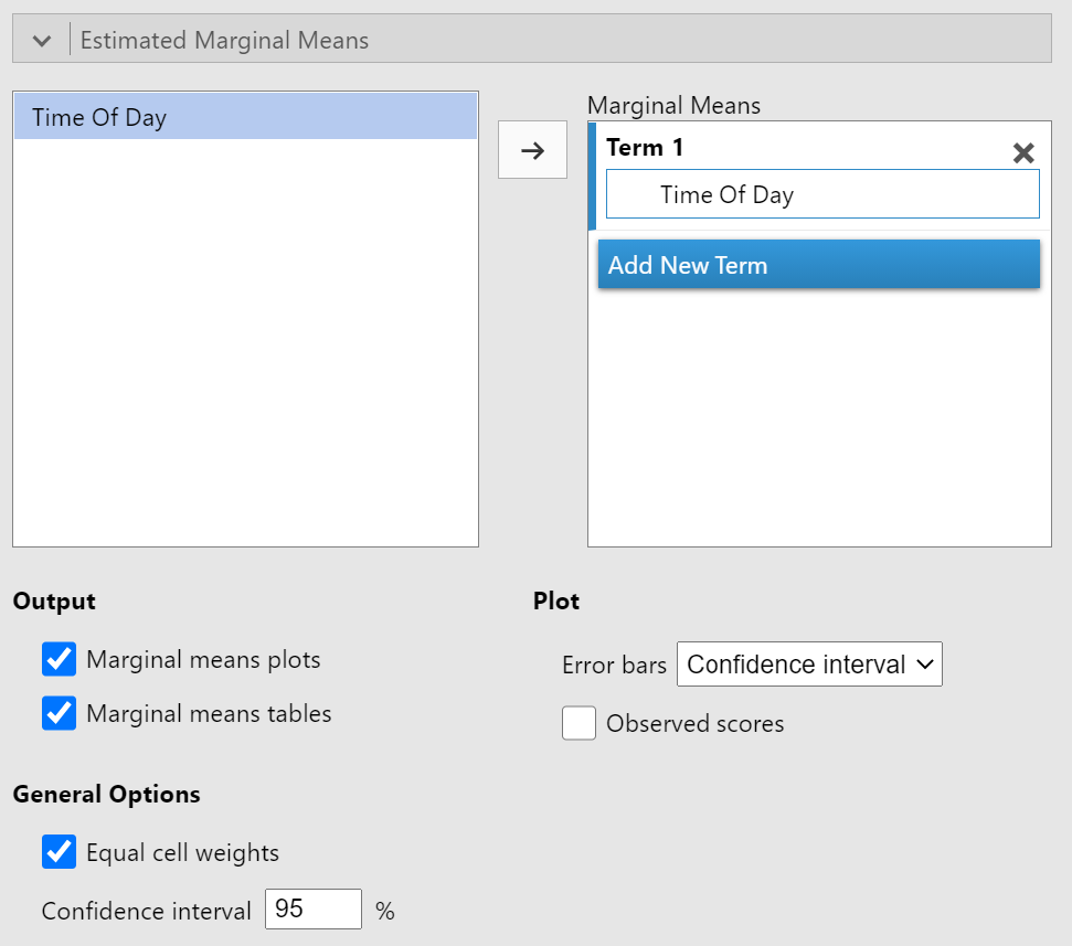
The last section that we will need to update is the "Estimated Marginal Means" section. Like the last section, we'll need to let jamovi know for which variables we want to calculate means and confidence intervals. Drag your within-subjects variable from the left side to the box under "Term 1" on the right side. Once that is set, make sure to turn on "Marginal means tables." You can find the completed "Estimated Marginal Means" section in Figure 15.
Figure 15
Completed Estimated Marginal Means Section
The ANOVA set up is complete and we're ready to interpret the results.
Interpreting the ANOVA Results
Mauchly's Test of Sphericity
We left one assumption unchecked because the test is included with the ANOVA. Let's go to the "Assumptions" section of the results and check on the "Tests of Sphericity" table (see Figure 16).
Figure 16
Test of Sphericity

Mauchly's test yielded a p-value less than α so we should reject the null hypothesis that sphericity (equal variance among difference scores) exists and that the assumption has been violated. This violation requires a correction. As outline above, we'll be using the Greenhouse-Geisser corrected values from the ANOVA table.
The ANOVA Table
This time, jamovi has prepared two tables for us. The first is the one of interest for this example: "Within Subjects Effects." The other table ("Between Subjects Effects") has some information about residuals (i.e., how different each participants overall averages are from the average of all participants) but we are not testing for any between-subjects variables.
Table 6 is a reproduction of the Within Subjects Effects table.
Table 6
Within Subjects Effects
| Effect | Sphericity Correction | Sum of Squares | df | Mean Square | F | p | η²p |
|---|---|---|---|---|---|---|---|
| Time Of Day | None | 10376 | 2 | 5188 | 12.9 | < .001 | 0.080 |
| Greenhouse-Geisser | 10376 | 1.06 | 9825 | 12.9 | < .001 | 0.080 | |
| Residual | None | 119524 | 298 | 401 | |||
| Greenhouse-Geisser | 119524 | 157.36 | 760 |
Note. Type 3 Sums of Squares
Because we had a violation of the assumption of sphericity, we need to focus on just the "Greenhouse-Geisser" rows. Table 7 is an updated version of the table with only the "Greenhouse-Geisser" rows.
Table 7
Greenhouse-Geisser Corrected Within Subjects Effects
| Effect | Sum of Squares | df | Mean Square | F | p | η²p |
|---|---|---|---|---|---|---|
| Time Of Day | 10376 | 1.06 | 9825 | 12.9 | < .001 | 0.080 |
| Residual | 119524 | 157.36 | 760 |
Note. Type 3 Sums of Squares and Greenhouse-Geisser corrected values.
Now we can interpret the results. The effect of "Time Of Day" yielded a statistically significant result because the p-value is less than α. We also see that the effect size (η²p) is .08, which is considered a "very small" effect according to table 7 from our last post.
With a small, but statistically significant effect of "Time of Day", we need to determine which times of day lead to reliably different happiness ratings with post-hoc analyses.
Bonferroni Tests
In the "Post Hoc Tests" section, you should see a table called "Post Hoc Comparisons - Time of Day" (see figure 17). This table has the comparisons of happiness ratings across each time of day. Importantly, each t-value has a corresponding pbonferroni value.
Table 17
Bonferroni Corrected Post Hoc Tests

With each comparison generating a pbonferroni < α, we can claim that the happiness rating for each time of day is reliably different from each other time of day.
Estimated Marginal Means
To make these differences more meaningful for our readers, let's make these comparisons using the original groupings and add some visuals. We can find the mean happiness rating (with 95% CI) in a table (table 8) and error bar plot (figure 18).
Table 8
Estimated Marginal Means for Time of Day
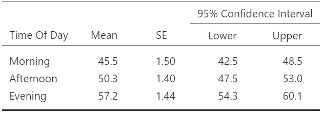
Interestingly, there is some overlap in the 95% CI for Morning and Afternoon (i.e., the upper bound of Morning is greater than the lower bound of Afternoon), despite there being a statistically significant difference reported in the post hoc tests. This is discrepancy occurs because the confidence interval calculation is based on the "uncorrected" standard errors. They are uncorrected in that the between-subjects variability has not been remove. As such, the 95% CI will be wider than the post-hoc tests.
Figure 18
Error Bar Plot for Time of Day
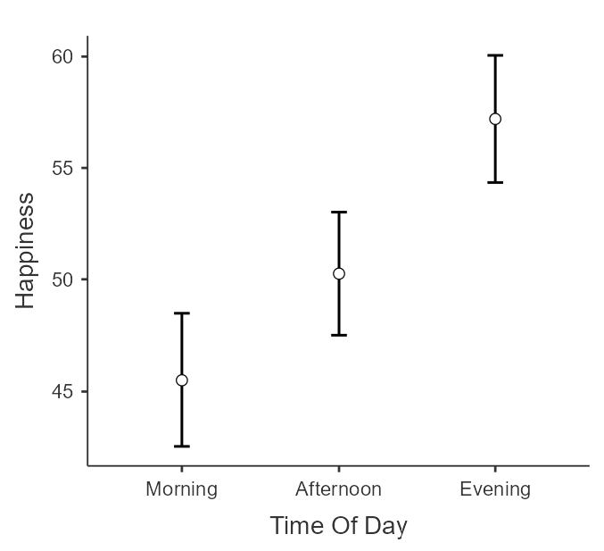
The table and figure indicate to us that individuals reported the greatest level of happiness in the evening followed by the afternoon with the lowest level of happiness in the morning.
In our write up, we'll want to combine information from our marginal means with our post hoc tests to describe the pattern of results (e.g., the ranking of results) with the reliability of differences.
Writing up the ANOVA results
Revisiting the Format
Recall from our write-up from the last post that we should have three components for each analyses we are writing-up.
- State the test
- Interpret the results
- Provide statistical evidence
Let's do this for each section of our analyses:
- Assumption checks
- One-Way Within-Subjects ANOVA
- Post hoc tests
The Write-Up
Let's combine the various pieces that we discussed in our review of the output.
"I assessed the normality and sphericity assumptions of the one-way within-subjects ANOVA. I calculated skewness and kurtosis statistics and examined Q-Q plots to assess normality of the samples. All samples had skewness values within 2 standard errors but the kurtosis values were above 3 standard errors (see table 1). A further examination of the Q-Q plots (see figure 1) indicated kurtosis but at a level that was within the robustness of ANOVA. Sphericity was assessed using Mauchly's test. The test revealed a violation of the assumption (W = 0.105, p < .001) so the Greenhouse-Geisser correction was used for the test of within-subjects effects of the ANOVA. There was a statistically significant but very small effect of Time of Day on Happiness (F[1.06,157.36] = 12.0, p < .001, η²p = .08). Bonferroni-corrected comparisons revealed that all comparisons were reliably different (see table 2). As can be seen in figure 2, happiness was lowest in the morning (M=45.5, 95% CI [42.5,48.5]), higher in the afternoon (M=50.3, 95% CI [47.5,53.0]), and highest in the evening (M=57.2, 95% CI [54.3,60.1])."
Table 1
Skewness and Kurtosis Values of Within-Subjects Samples

Table 2 Bonferroni-corrected Comparisons

Figure 1
Q-Q Plots of Within-Subjects Samples


Summary
In this lesson, we:
- Explored the process of the within-subjects ANOVA,
- Compared the between- to the within-subjects ANOVA,
- Stated the goals and assumptions of the within-subjects ANOVA,
- Conducted a repeated measures ANOVA for the one-way within-subjects ANOVA,
- Interpreted the results of the repeated measures ANOVA,
- Made conclusions based on the post hoc tests, and
- Presented the results in APA format.
In the next lesson, we’re back to between-subjects designs but we are increasing the complexity. The factorial between-subjects ANOVA addresses multiple independent variables.